0. Summary
- Topic modeling : corpus 집합에서 통계적 분석 방식을 사용해서 문서의 context를 담고 있는 유의미한 word를 뽑아내고 representation 만들기.
- DTM : Document-Term Matrix / 문서 단어 행렬
- 키워드로 보는 Method
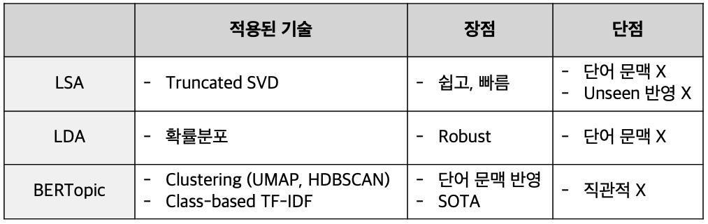
- LSA : #유사도, #토픽 모델링 아이디어 시초 #SVD
- LDA : #확률분포, #문서별 토픽분포 추가
- BERTopic : #SOTA, #clustering, #class-based TF-IDF, #BERT
- keypoint!
- 각 method별 한계와 극복 방법 + 최신엔 어떤 걸 쓰고 있나?
- LSA paper : Landauer, T. K., Foltz, P. W., & Laham, D. (1998). An introduction to latent semantic analysis. Discourse processes, 25(2-3), 259-284.
- LDA paper : Blei, D. M., Ng, A. Y., & Jordan, M. I. (2003). Latent dirichlet allocation. Journal of machine Learning research, 3(Jan), 993-1022.
- BERTopic paper: BERTopic: Neural topic modeling with a class-based TF-IDF procedure
1. LSA (Latent Semantic Analysis)
1-1. background
- Bag of words, TF-IDF는 단어 빈도수 기반으로 수치화 했기 때문에 단어의 의미는 고려하지 못한다는 단점이 있었음. (= 단어의 토픽을 고려하지 못한다.)
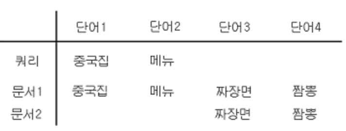
키워드 매칭만 생각했을 때 '중국집' 단어는 문서 1이랑만 매칭돼서, 문서2는 검색에서 빠져버리게 된다.
1-2. Approach
-
Co-occurrence를 통해 DTM의 잠재된(latent) 의미를 이끌어 내자
co-occurrence 정보를 이용한다 == semantic을 이용한다 !!
위의 예시에서 문서1 상 '중국집'은 '짜장면', '짬뽕'과 동시 등장함. 이를 통해 문서 2도 비슷하지 않을까! 하는 사실을 유추해볼 수 있음. -
차원 축소 : Truncated SVD
1-3. Method
Full SVD (Singular Value Decomposition, 특이값 분해)
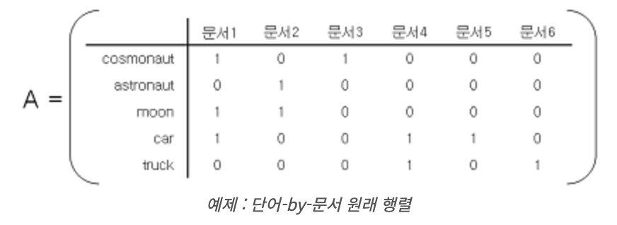
- m x n 행렬 A를 3개의 행렬 곱으로 분해
- 특징 : 세개 다 합치면 다시 원래 행렬인 A로 돌아감
- 원래 행렬 A
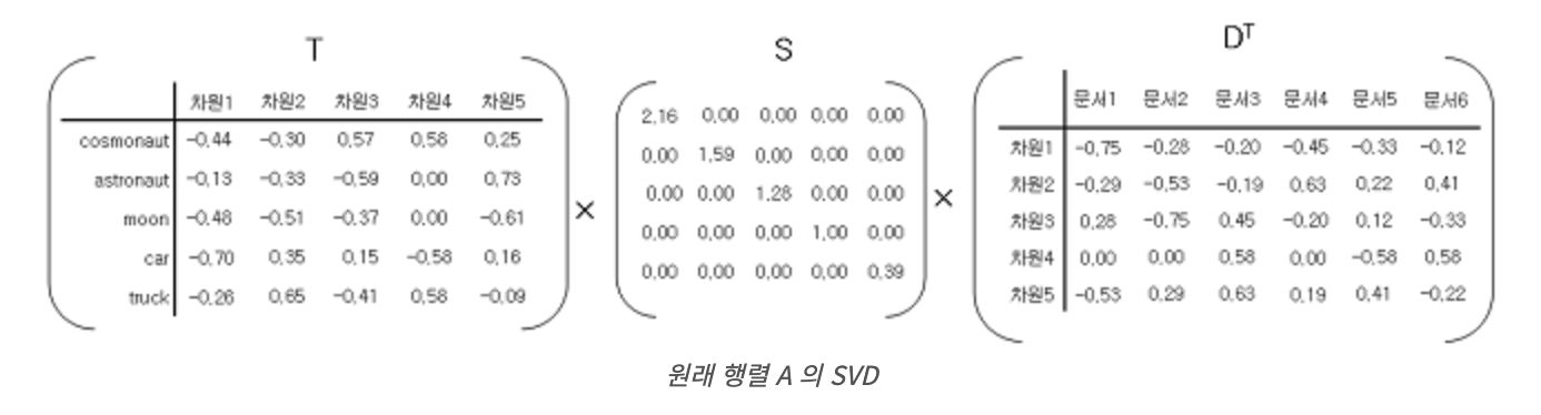
- 분해된 행렬
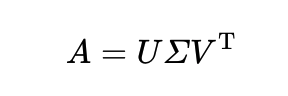
- 수식

- U: 직교 행렬 (m x m) - 자기 자신과 전치행렬 곱했을 때 단위행렬 나오는 경우
- V: 직교 행렬 (n x n)
- E: 직사각 대각 행렬 (m x n) - 주대각선을 제외한 곳 원소 모두 0인 행렬
*A의 특이값(singular value): 대각행렬 S에서 나온 대각 원소의 값
- 원래 행렬 A
Truncated SVD (LSA method!)
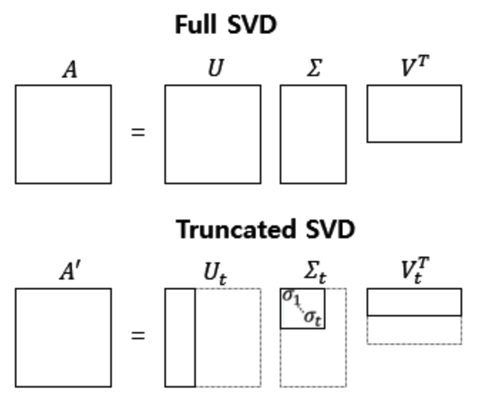
- Full SVD의 3개 행렬에서 일부 벡터 삭제하고 절단된(truncated) SVD만 사용 (상위 t개 선택).
- 절단 되면 대각 원소 값 중에서 상위 t개만 남게 된다.
- t : 뽑고자 하는 토픽 수 (t 크게 잡으면 기존 행렬 의미는 다양하게 담을 수 있으나, 작게 잡아야 노이즈 제거할 수 있음)
- 특징
- 값 손실이 있어서 원래 행렬 A로는 복구할 수 X
- 데이터 차원을 줄여서 Full SVD보다 계산 비용 낮아짐
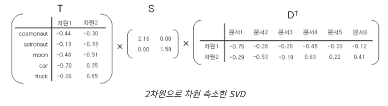
Latent Semantic Analysis
- T x S : 단어-단어 간의 유사도 계산
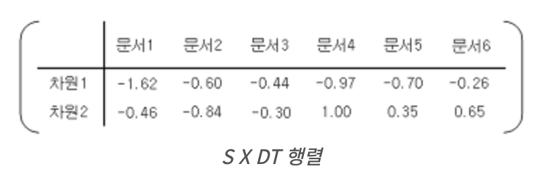
- S x D^T : 문서 - 문서 간의 유사도 계산
- T x S x D^T : 단어 - 문서간의 유사도 계산
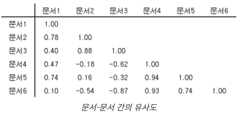
문서-문서 유사도 예시
- 문서 1과 문서2간 유사도 : arr[:,1] , arr[:,2] 간 cosine similarity 계산
- 문서 4,5 간 유사도 높은 것 확인
1-4. LSA의 특징
- 장점
- 쉽고, 빠르게 구현
- 단어의 잠재적 의미 이끌어내어 문서 유사도 계산에서 good
- 단점
- 이미 계산된 LSA에 새로운 데이터 추가하여 계산 X, 처음부터 다시 계산
- 단어 순서 고려하지 않음.
- still be suspected of resulting incompleteness or likely error on some occasions
2. LDA (Latent Dirichlet Allocation)
Ref :
2-1. background
- LSA 이후 pLSA (Probabilistic LSA)가 나옴
- 문서 내 단어가 등장할 확률을 기반으로 DTM 구성.
- 확률값이 나와야하기 때문에 SVD 사용 X (SVD는 0~1 아닌 값도 나오기 때문)
- Non-negative Matrix Factorization(NMF,음수 미포함 행렬 분해) or Expectation-maximization algorithm (기대값 최대화 기법) 등을 활용해 행렬 분해
- 한계점
- LSA처럼 토픽별로 어떤 단어를 가지고 있는지는 볼 수 있는데 문서별로 어떤 주제가 분포하고 있는지는 활용하지 않는다.
- 새로운 문서에 대해서는 토픽 뽑기 어려움
2-2. Approach
- pLSA 단점 보완 : 토픽별 단어 분포 + 문서별 토픽 분포까지
- 단어가 특정 토픽에 존재할 확률 + 특정 토픽이 특정 문서에 존재할 확률 모두 사용
- 문서들은 토픽들의 혼합으로 구성되어 있고, 토픽들은 확률 분포에 기반하여 단어들을 생성한다고 가정
- Collapsed gibbs sampling (깁스 샘플링)
2-3. Method
- 주어진 문서에 대하여 각각 어떤 주제들이 존재하는지 구하는 확률 모델.
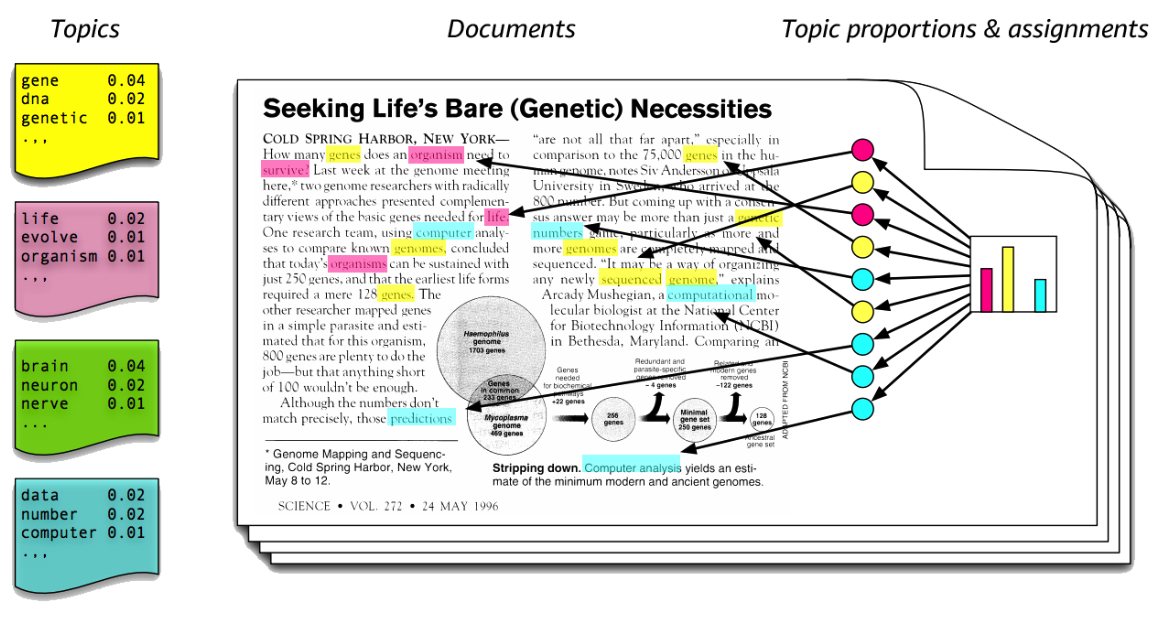
- 노란색 토픽엔 gene ,,,등의 단어 존재
- 오른쪽 문서에는 노란색 토픽과 관련한 단어 수 많음 == 노란색 토픽일 확률 높음.
Architecture
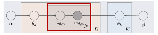
- 1) Notation
- observed word (w_d,n) : d번째 문서의 n번째 단어
- 네모 박스 : 반복해라
- 동그라미 : 변수
- 화살표 : 조건 -> 결과
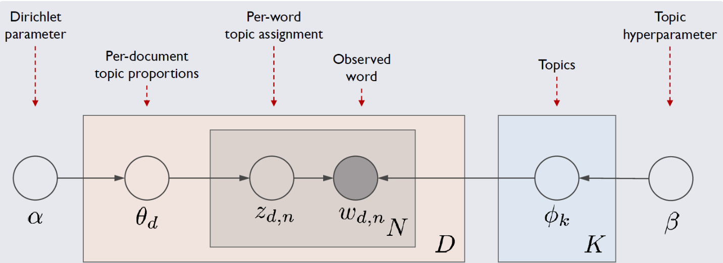
- 2) 구조
: LDA가 가정하는 문서가 생성되는 과정을 확률 모형으로 모델링
(e.g., 어떤 토픽으로 쓸 지 고른 후, 토픽에 해당하는 단어들을 이용해 문장을 생성)- α:Dirichlet parameter
- e.g. 1번째 문서에서 topic2에 할당된 단어들이 하나도 없을 수도 있기 때문에 이를 위해 일종의 smoothing하는 역할을 해줌. 따라서 A가 아예 0인 경우는 안나옴. α가 클수록 토픽들의 분포가 비슷해지고, 작을 수록 특정 토픽만 크게 나옴(횟수에 따라)
- β:Topic hyperparameter
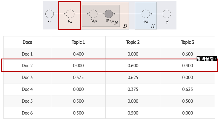
- θ𝑑: d번째 문서 벡터 (1 X 토픽 수)
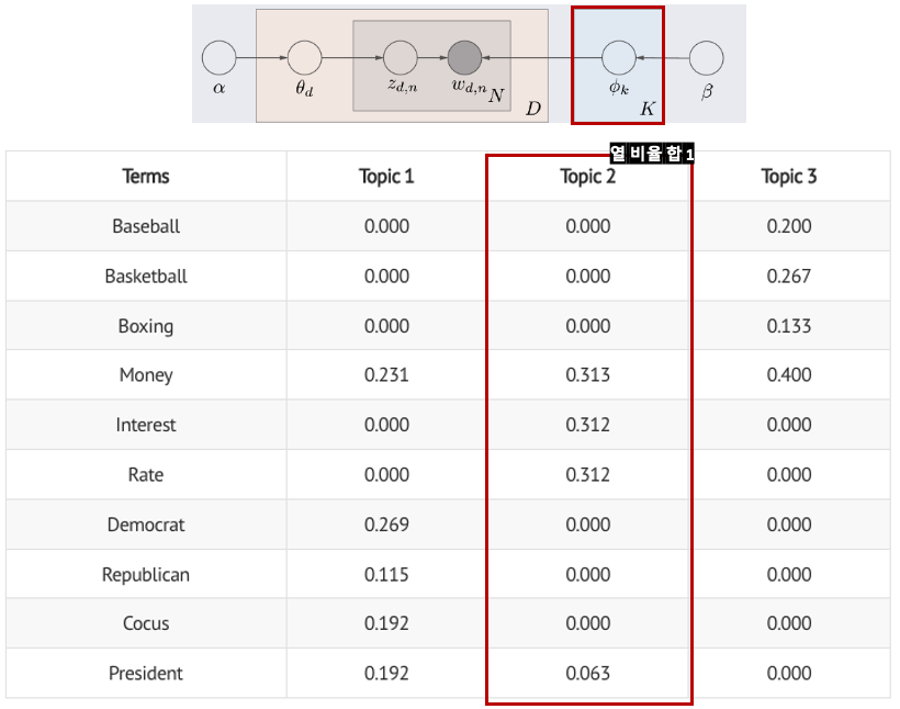
- ϕ𝑘: k번째 토픽 벡터 (1 X 단어 수)
- 𝑧𝑑,𝑛 : d번째 문서 n번째 단어가 어떤 토픽에 해당하는지 할당 (θ𝑑 영향)
- e.g., Doc2의 1번째 단어는 Topic2일 확률이 가장 높음. z_2,1 = Topic 2
- 𝑤𝑑,𝑛 : d번째 문서 n번째 단어에 특정 단어를 할당 (ϕ𝑘 와 𝑧𝑑,𝑛에 동시에 영향)
- e.g., z_2,1 = Topic 2 이기 때문에 ϕ2 벡터를 확인 함. ϕ2에서 Money의 확률이 가장 높기 때문에 w_2,1 = Money
- e.g., z_2,1 = Topic 2 이기 때문에 ϕ2 벡터를 확인 함. ϕ2에서 Money의 확률이 가장 높기 때문에 w_2,1 = Money
- 이 과정을 네모 상자에 써진 N,D,K 번 만큼 반복해서 실행.
- 최종적으로 LDA는 토픽의 단어분포(ϕ𝑘)와 문서의 토픽분포(θ𝑑)의 결합으로 문서 내 단어들이 생성된다고 가정
- α:Dirichlet parameter
LDA learning & inference
-
Goal: 위의 문서생성 과정을 역으로 따라가서 𝑤𝑑,𝑛 를 가지고 잠재변수를 추정 (z, ϕ, θ)
( ~ 단어를 보고 어떤 토픽 분포에서 왔는지 추정, 이 토픽을 보고 어떤 문서 분포에서 왔는지 추정)
-
Collapsed gibbs sampling (깁스 샘플링)
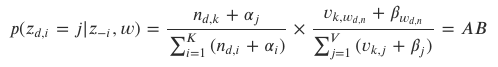
- 단어 w는 잘못된 토픽에 할당되어 있고, 나머지는 올바르게 할당되어 있다고 가정해서 w의 정보를 제외한 다른 정보를 이용해서 w의 토픽 할당
- 𝑝(𝑧𝑖=𝑗|𝑧−𝑖,𝑤) : w (observed word)와 𝑧−𝑖 (i번째 단어의 토픽 정보를 제외한 모든 단어의 토픽 정보)가 주어졌을 때 i번째 단어의 토픽이 j일 확률
-
Process
-
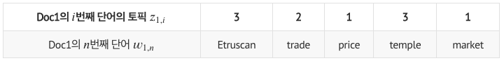
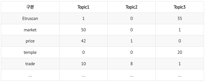
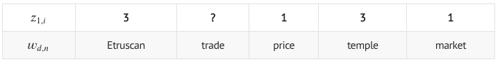
0) 목표 : 𝑝(𝑧_1,2) 구하기! (1번째 문서의 2번째 단어 'trade'의 토픽 구하기)
-
1) 𝑧𝑖, ϕ𝑘 랜덤 초기화, 토픽 수(k) 지정
-
2) 깁스 샘플링 활용해 𝑝(𝑧_1,2) 구하기
-
target 단어 ('trade')의 정보만 지우고 나머지 정보만 활용
-
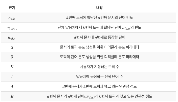
A : 𝑑번째 문서가 𝑘번째 토픽과 맺고 있는 연관성 정도
- p(topic|doc d) : doc d에 포함된 단어들의 토픽 할당 비율 계산 (특정 문서는 어떤 토픽으로 주로 이루어져 있나?)
- e.g., 𝑛_1,1=2, 𝑛_1,3=2
예시 : 1번째 문서의 토픽별 연관성 정도(A)

-
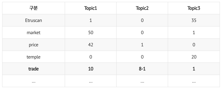
B : 𝑑번째 문서의 𝑛번째 단어(𝑤𝑑,𝑛)가 𝑘번째 토픽과 맺고 있는 연관성 정도
- p(word w|topic) : 각 토픽마다 단어 w의 분포 계산 (타겟 단어는 전체 문서에서 주로 어떤 토픽으로 할당되었었나?)
- 깁스 샘플링으로 인해 trade의 토픽 정보가 지워져서, 단어별 토픽 분포 표에 반영됨

- e.g., 𝑣_1,𝑡𝑟𝑎𝑑𝑒 =10 , 𝑣_2,𝑡𝑟𝑎𝑑𝑒=7, 𝑣_3,𝑡𝑟𝑎𝑑𝑒=1
예시: trade 단어의 토픽별 연관성 정도(B)
-
𝑝(𝑧_1,2) == AB
- 이와 같은 상황에서 z_1,2는 넓이가 가장 큰 topic 1로 할당될 가능성 가장 큼
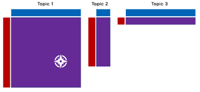
- 이와 같은 상황에서 z_1,2는 넓이가 가장 큰 topic 1로 할당될 가능성 가장 큼
-
-
3) 2번 반복 수행
- 2번 반복하여 θ, ϕ 계속 업데이트 (보통 1000~1만회 반복)
-
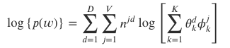
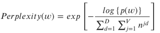
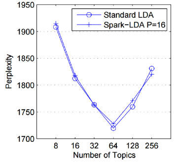
최적의 토픽 수 K 찾기 (perplexity)
- 모든 토픽에 대한 합 계산, perplexity가 가장 낮은 k로 토픽 수 지정
- ϕ와 θ의 곱을 이용해서 단어의 발생확률 이용 p(w)는 높을 수록 good
- 대략 여기까지만...
2-4. LDA 특징
-
장점: 가정이 위반되더라도 어느정도 robust (변화에 민감하지 않다).
출처: https://mambo-coding-note.tistory.com/205 [화학쟁이의 ㎚코딩노트:티스토리] -
단점:
- DTM/TF-IDF를 입력으로 받기 때문에 여전히 LDA도 단어 순서 신경쓰지 X
- 가장 작은 그룹의 샘플 수가 설명변수의 개수보다 많아야 함.
- 정규분포 가정에 크게 벗어난다면, 잘 설명하지 못한다.
- 공분산 구조가 서로 다른 경우를 반영하지 못한다.
출처: https://mambo-coding-note.tistory.com/205 [화학쟁이의 ㎚코딩노트:티스토리]
=> 단점 보완해서 등장한 것이 QDA (Quadratic Discriminant Analysis)라고 함
3. BERTopic
3-1. background
- LDA 단어 순서 신경쓰지 X, 단어의 문맥 정보를 고려하지 않으면 document를 제대로 represent할 수 없음.
- LDA는 확률분포로 토픽 추정했지만, 문맥 파악 관점에서 최근엔 topic modeling을 clustering task로 접근하는 경우 많아짐 (Top2Vec - Doc2Vec 임베딩 사용, HDBSCAN)
- 하지만, a cluster will not always lie within a sphere around a cluster centroid (the centroid-based perspective 문제).
3-2. Approach
- 1) contextual word & sentence vector 를 뽑는 BERT 활용해 document 단위로 embedding 추출해서 클러스터링
- 2) Clustering을 통해 차원 축소
- 3) class-based TF-IDF를 이용해 topic representation 생성
3-3. Method
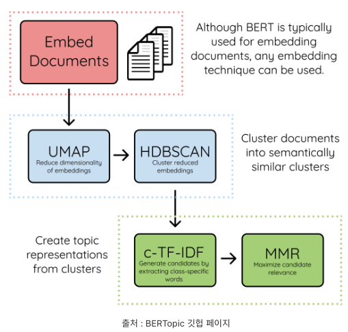
1) Document Embeddings
- pretrained 모델 사용
- default
- "all-MinLM-L6-v2" (영어)
- "paraphrase-multilingual-MinLm-L12-v2" (50+ other languages)
2) Document Clustering
- UMAP (Uniform Manifold Approximation and Projection)
- 목적 : 임베딩의 local 및 global structure을 보존하면서 차원 축소
- method : neighbor graph 기반
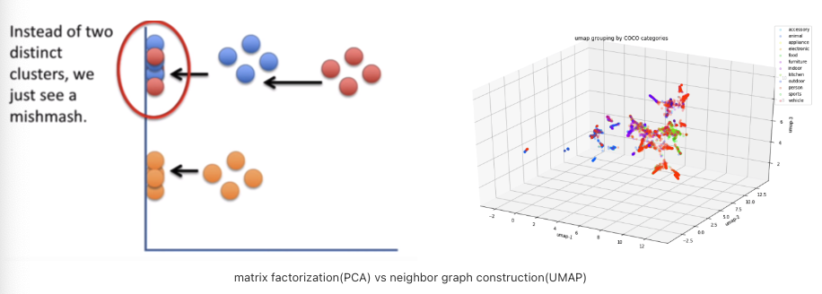
- PCA : matrix factorization
- t-SNE : neighbor graph
- HDBSCAN (Hierarchical DBSCAN)
- UMAP을 통해 축소된 임베딩을 HDBSCAN 사용해 outlier 식별하고 클러스터링.
- DBSCAN :
- 고차원의 nested clusters를 효과적으로 분류하기 위해 고안된 알고리즘
- density 기반 single-linkage 클러스터링 이용해 클러스터 간 위계 구성(hierarchical)
- DBSCAN 클러스터는 density-connected point들을 최대로 포함하는 집합으로 정의
- DBSCAN :
- UMAP을 통해 축소된 임베딩을 HDBSCAN 사용해 outlier 식별하고 클러스터링.
3) Topic representation
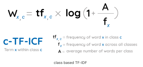
- class-based TF-IDF : 구성된 클러스터들 안에서, 클러스터와 클러스터를 구분하기 위함.
- 단일 클러스터의 모든 문서를 단일 문서로 간주하고 TF-IDF 적용
- 산출된 matrix의 각 행은 해당 클러스터 내의 단어에 대한 중요도 점수
- 클러스터 별 가장 중요한 단어 산출
3-4. BERTopic 특징
- 장점
- BERTopic은 LDA를 견줄만한 Topic modeling이라고 칭송 받는다고 함.
- embedding 과정과 representation이 독립적으로 있기 때문에 다양한 varation을 줄 수 있음.
- class-based version of TF-IDF를 사용하면 하나의 문서에 대한 토픽만 보는 것이 아니라 전체 class (cluster) 안에서의 토픽 representation을 뽑을 수 있다. (좀 더 전체적인 context를 볼 수 있다는 것이겠지??)
- 단점
- 하나의 document는 하나의 topic만 가진다고 가정한다. 그래서 multiple topic을 반영하기 힘들 수도 있다.
- 전체적인 문맥을 반영한다고는 하나 topic representation이 BoW 방식에서 생성된 것 만큼 직관적으로 설명되진 않을 수 있고 중복 같은 게 발생할 수 있다. (LDA 같은 경우는 topic을 10개 이런식으로 지정해서 만드는데 BERTopic은 autho로 설정하면 막 140개의 토픽이 나와버림)
4. Conclusion
4-1. Summary
** 참고 : KeyBERT
https://heeya-stupidbutstudying.tistory.com/entry/DL-keyword-extraction-with-KeyBERT-%EA%B0%9C%EC%9A%94%EC%99%80-%EC%95%8C%EA%B3%A0%EB%A6%AC%EC%A6%98-1
BERTopic과 같은 개발자
4-2. 느낀점
- Topic Modeling은 그냥 LDA! 라고만 생각했는데..... 이 정도로 넓은 세계인 줄 몰랐다. 우리가 아는 것은 정말 지구 크기에서 개미 하나 본 것 뿐이었던 것이었던 것이었다.....
- 데이터 마이닝 관점에서 topic modeling은 LDA가 아직까진 간편하게 사용할 수 있으니 좋은 것 같음!
- 그런데, keyword를 활용해 knowledge graph를 만든다는 가 Entity를 뽑는다든가의 task를 위해서는 SOTA를 사용 or dataset의 특징에 맞는 model을 사용해야겠다!
5. Implementation
- LSA
- LDA
- KeyBERT
1. LSA
- ref : https://wikidocs.net/24949
- Full SVD
- Truncated SVD
- Library
1) Full SVD - From scratch
import numpy as np

# DTM 정의
# 문서 단어 행렬(Document-Term Matrix, DTM)

A = np.array([[0,0,0,1,0,1,1,0,0],
              [0,0,0,1,1,0,1,0,0],
              [0,1,1,0,2,0,0,0,0],
              [1,0,0,0,0,0,0,1,1]])

print('DTM의 크기(shape) :', np.shape(A))
DTM의 크기(shape) : (4, 9)"""
U, S, V
linalg.svd()
"""
U, s, VT = np.linalg.svd(A, full_matrices = True)
print(f'행렬 U : [shape: {np.shape(U)}]')
print(U.round(2))행렬 U : [shape: (4, 4)]
[[-0.24 0.75 0. -0.62]
[-0.51 0.44 -0. 0.74]
[-0.83 -0.49 -0. -0.27]
[-0. -0. 1. 0. ]]# 특이값 벡터 리스트 => 대각 행렬로 변형
print(f'특이값 벡터 리스트 s : [shape: {np.shape(s)}]')
print(s.round(2))
print()
S = np.zeros((4, 9)) # 대각 행렬의 크기인 4 x 9의 임의의 행렬 생성
S[:4, :4] = np.diag(s) # 특이값을 대각행렬에 삽입
print(f'대각행렬 S : [shape: {np.shape(S)}]')
print(S.round(2))특이값 벡터 리스트 s : [shape: (4,)]
[2.69 2.05 1.73 0.77]
대각행렬 S : [shape: (4, 9)]
[[2.69 0. 0. 0. 0. 0. 0. 0. 0. ]
[0. 2.05 0. 0. 0. 0. 0. 0. 0. ]
[0. 0. 1.73 0. 0. 0. 0. 0. 0. ]
[0. 0. 0. 0.77 0. 0. 0. 0. 0. ]]print(f'직교행렬 VT : [shape: {np.shape(VT)}]')
print(VT.round(2))직교행렬 VT : [shape: (9, 9)]
[[-0. -0.31 -0.31 -0.28 -0.8 -0.09 -0.28 -0. -0. ]
[ 0. -0.24 -0.24 0.58 -0.26 0.37 0.58 -0. -0. ]
[ 0.58 -0. 0. 0. -0. 0. -0. 0.58 0.58]
[ 0. -0.35 -0.35 0.16 0.25 -0.8 0.16 -0. -0. ]
[-0. -0.78 -0.01 -0.2 0.4 0.4 -0.2 0. 0. ]
[-0.29 0.31 -0.78 -0.24 0.23 0.23 0.01 0.14 0.14]
[-0.29 -0.1 0.26 -0.59 -0.08 -0.08 0.66 0.14 0.14]
[-0.5 -0.06 0.15 0.24 -0.05 -0.05 -0.19 0.75 -0.25]
[-0.5 -0.06 0.15 0.24 -0.05 -0.05 -0.19 -0.25 0.75]]# (4,4) X (4,9) X (9,9)
print(f'USV^T : [shape: {np.shape(np.dot(np.dot(U,S), VT))}]')
print(f'DTM: [shape: {np.shape(A)}]')
np.allclose(A, np.dot(np.dot(U,S), VT).round(2))USV^T : [shape: (4, 9)]
DTM: [shape: (4, 9)]
True2) Truncated SVD
- topic 수 t 고정 (t = 2)
S = S[:2,:2] # 특이값 상위 2개만 보존
U = U[:,:2]
VT = VT[:2,:]

print(f'행렬 U : [shape: {np.shape(U)}]')
print(f'대각행렬 S : [shape: {np.shape(S)}]')
print(f'직교행렬 VT : [shape: {np.shape(VT)}]')
행렬 U : [shape: (4, 2)]
대각행렬 S : [shape: (2, 2)]
직교행렬 VT : [shape: (2, 9)]# (4,2) X (2,2) X (2,9)
# U 4X2 : 문서의 개수 X 토픽 수 t => 단어 갯수 9개는 유지 X, 문서크기 4 유지/ 4개의 문서를 각각 2개의 값으로 표현
# VT 2X9 : t X 단어수 => 잠재의미를 표현하는 단어 벡터
print(f'축소된 USV^T : [shape: {np.shape(np.dot(np.dot(U,S), VT))}]')
print(f'DTM: [shape: {np.shape(A)}]')
np.allclose(A, np.dot(np.dot(U,S), VT).round(2))축소된 USV^T : [shape: (4, 9)]
DTM: [shape: (4, 9)]
False3) Library 사용
- DTM 만들기 : tf-idf
- Topic modeling : TruncatedSVD
import pandas as pd
from sklearn.datasets import fetch_20newsgroups
import nltk
from nltk.corpus import stopwords
from sklearn.feature_extraction.text import TfidfVectorizer
from sklearn.decomposition import TruncatedSVD
### data load
dataset = fetch_20newsgroups(shuffle=True,
random_state=1,
remove=('headers', 'footers', 'quotes'))
documents = dataset.data
print('샘플 수:',len(documents))
print(dataset.target_names, len(dataset.target_names)) # topic 주제
documents[1]샘플 수: 11314
['alt.atheism', 'comp.graphics', 'comp.os.ms-windows.misc', 'comp.sys.ibm.pc.hardware', 'comp.sys.mac.hardware', 'comp.windows.x', 'misc.forsale', 'rec.autos', 'rec.motorcycles', 'rec.sport.baseball', 'rec.sport.hockey', 'sci.crypt', 'sci.electronics', 'sci.med', 'sci.space', 'soc.religion.christian', 'talk.politics.guns', 'talk.politics.mideast', 'talk.politics.misc', 'talk.religion.misc'] 20
"\n\n\n\n\n\n\nYeah, do you expect people to read the FAQ, etc. and actually accept hard\natheism? No, you need a little leap of faith, Jimmy. Your logic runs out\nof steam!\n\n\n\n\n\n\n\nJim,\n\nSorry I can't pity you, Jim. And I'm sorry that you have these feelings of\ndenial about the faith you need to get by. Oh well, just pretend that it will\nall end happily ever after anyway. Maybe if you start a new newsgroup,\nalt.atheist.hard, you won't be bummin' so much?\n\n\n\n\n\n\nBye-Bye, Big Jim. Don't forget your Flintstone's Chewables! :) \n--\nBake Timmons, III"### data preprocessing
news_df = pd.DataFrame({'document':documents})
news_df['clean_doc'] = news_df['document'].str.replace("[^a-zA-Z]", " ") # 특문
news_df['clean_doc'] = news_df['clean_doc'].apply(lambda x: ' '.join([w for w in x.split() if len(w)>3]))
news_df['clean_doc'] = news_df['clean_doc'].apply(lambda x: x.lower())
news_df['clean_doc'][1]
stop_words = stopwords.words('english') # stopwords
tokenized_doc = news_df['clean_doc'].apply(lambda x: x.split())
tokenized_doc = tokenized_doc.apply(lambda x: [item for item in x if item not in stop_words])
print(tokenized_doc[1])
# 역토큰화 (토큰화 작업을 역으로 되돌림)
detokenized_doc = []
for i in range(len(news_df)):
t = ' '.join(tokenized_doc[i])
detokenized_doc.append(t)
news_df['clean_doc'] = detokenized_doc
news_df['clean_doc'][1]/tmp/ipykernel_1097416/312981451.py:3: FutureWarning: The default value of regex will change from True to False in a future version.
news_df['clean_doc'] = news_df['document'].str.replace("[^a-zA-Z]", " ") # 특문
['yeah', 'expect', 'people', 'read', 'actually', 'accept', 'hard', 'atheism', 'need', 'little', 'leap', 'faith', 'jimmy', 'logic', 'runs', 'steam', 'sorry', 'pity', 'sorry', 'feelings', 'denial', 'faith', 'need', 'well', 'pretend', 'happily', 'ever', 'anyway', 'maybe', 'start', 'newsgroup', 'atheist', 'hard', 'bummin', 'much', 'forget', 'flintstone', 'chewables', 'bake', 'timmons']
'yeah expect people read actually accept hard atheism need little leap faith jimmy logic runs steam sorry pity sorry feelings denial faith need well pretend happily ever anyway maybe start newsgroup atheist hard bummin much forget flintstone chewables bake timmons'news_df.head(2)| document | clean_doc | |
|---|---|---|
| 0 | Well i'm not sure about the story nad it did s... | well sure story seem biased disagree statement... |
| 1 | \n\n\n\n\n\n\nYeah, do you expect people to re... | yeah expect people read actually accept hard a... |
### TF-IDF
vectorizer = TfidfVectorizer(stop_words='english',
                             max_features= 1000, # 상위 1,000개의 단어를 보존
                             max_df = 0.5,
                             smooth_idf=True)

X = vectorizer.fit_transform(news_df['clean_doc'])

print('TF-IDF 행렬의 크기 :',X.shape) ## == DTM
TF-IDF 행렬의 크기 : (11314, 1000)### Topic modeling
"""
TruncatedSVD(n_components=2, *, algorithm='randomized', n_iter=5, random_state=None,tol=0.0,)
- n_components : Desired dimensionality of output data.
- algorithm : SVD solver to use. {'arpack', 'randomized'}, default='randomized'
- n_iter : Number of iterations for randomized SVD solver
- tol : Tolerance for ARPACK. 0 means machine precision.
"""
svd_model = TruncatedSVD(n_components=20, # topic 수
algorithm='randomized',
n_iter=100,
random_state=122)
svd_model.fit(X)
print("topic 수 : ",len(svd_model.components_))
print(np.shape(svd_model.components_))topic 수 : 20
(20, 1000)terms = vectorizer.get_feature_names() # 단어 집합. 1,000개의 단어가 저장됨.
def get_topics(components, feature_names, n=5):
for idx, topic in enumerate(components):
print("Topic %d:" % (idx+1), [(feature_names[i], topic[i].round(5)) for i in topic.argsort()[:-n - 1:-1]])
get_topics(svd_model.components_,terms)Topic 1: [('like', 0.21386), ('know', 0.20046), ('people', 0.19293), ('think', 0.17805), ('good', 0.15128)]
Topic 2: [('thanks', 0.32888), ('windows', 0.29088), ('card', 0.18069), ('drive', 0.17455), ('mail', 0.15111)]
Topic 3: [('game', 0.37064), ('team', 0.32443), ('year', 0.28154), ('games', 0.2537), ('season', 0.18419)]
Topic 4: [('drive', 0.53324), ('scsi', 0.20165), ('hard', 0.15628), ('disk', 0.15578), ('card', 0.13994)]
Topic 5: [('windows', 0.40399), ('file', 0.25436), ('window', 0.18044), ('files', 0.16078), ('program', 0.13894)]
Topic 6: [('chip', 0.16114), ('government', 0.16009), ('mail', 0.15625), ('space', 0.1507), ('information', 0.13562)]
Topic 7: [('like', 0.67086), ('bike', 0.14236), ('chip', 0.11169), ('know', 0.11139), ('sounds', 0.10371)]
Topic 8: [('card', 0.46633), ('video', 0.22137), ('sale', 0.21266), ('monitor', 0.15463), ('offer', 0.14643)]
Topic 9: [('know', 0.46047), ('card', 0.33605), ('chip', 0.17558), ('government', 0.1522), ('video', 0.14356)]
Topic 10: [('good', 0.42756), ('know', 0.23039), ('time', 0.1882), ('bike', 0.11406), ('jesus', 0.09027)]
Topic 11: [('think', 0.78469), ('chip', 0.10899), ('good', 0.10635), ('thanks', 0.09123), ('clipper', 0.07946)]
Topic 12: [('thanks', 0.36824), ('good', 0.22729), ('right', 0.21559), ('bike', 0.21037), ('problem', 0.20894)]
Topic 13: [('good', 0.36212), ('people', 0.33985), ('windows', 0.28385), ('know', 0.26232), ('file', 0.18422)]
Topic 14: [('space', 0.39946), ('think', 0.23258), ('know', 0.18074), ('nasa', 0.15174), ('problem', 0.12957)]
Topic 15: [('space', 0.31613), ('good', 0.3094), ('card', 0.22603), ('people', 0.17476), ('time', 0.14496)]
Topic 16: [('people', 0.48156), ('problem', 0.19961), ('window', 0.15281), ('time', 0.14664), ('game', 0.12871)]
Topic 17: [('time', 0.34465), ('bike', 0.27303), ('right', 0.25557), ('windows', 0.1997), ('file', 0.19118)]
Topic 18: [('time', 0.5973), ('problem', 0.15504), ('file', 0.14956), ('think', 0.12847), ('israel', 0.10903)]
Topic 19: [('file', 0.44163), ('need', 0.26633), ('card', 0.18388), ('files', 0.17453), ('right', 0.15448)]
Topic 20: [('problem', 0.33006), ('file', 0.27651), ('thanks', 0.23578), ('used', 0.19206), ('space', 0.13185)]LDA
- ref : https://wikidocs.net/30708
- Sklearn library 사용
- gensim library 사용
tokenized_doc[:5]0 [well, sure, story, seem, biased, disagree, st...
1 [yeah, expect, people, read, actually, accept,...
2 [although, realize, principle, strongest, poin...
3 [notwithstanding, legitimate, fuss, proposal, ...
4 [well, change, scoring, playoff, pool, unfortu...
Name: clean_doc, dtype: object1) sklearn
from sklearn.decomposition import LatentDirichletAllocation
lda_model = LatentDirichletAllocation(n_components=10,
                                      learning_method='online',
                                      random_state=777,
                                      max_iter=1)
2) gensim
# 1) 정수 인코딩과 단어 집합 만들기

from gensim import corpora
dictionary = corpora.Dictionary(tokenized_doc)
corpus = [dictionary.doc2bow(text) for text in tokenized_doc]
print("encoding된 corpus 1 예시: \n", corpus[1]) # 수행된 결과에서 두번째 뉴스 출력. 첫번째 문서의 인덱스는 0
print("66번째 dictionary 예시:", dictionary[66])
print("학습된 총 단어의 갯수: ",len(dictionary))
encoding된 corpus 1 예시:
[(52, 1), (55, 1), (56, 1), (57, 1), (58, 1), (59, 1), (60, 1), (61, 1), (62, 1), (63, 1), (64, 1), (65, 1), (66, 2), (67, 1), (68, 1), (69, 1), (70, 1), (71, 2), (72, 1), (73, 1), (74, 1), (75, 1), (76, 1), (77, 1), (78, 2), (79, 1), (80, 1), (81, 1), (82, 1), (83, 1), (84, 1), (85, 2), (86, 1), (87, 1), (88, 1), (89, 1)]
66번째 dictionary 예시: faith
학습된 총 단어의 갯수: 64281# 2) LDA 모델 훈련시키기
import gensim
NUM_TOPICS = 20 # 20개의 토픽, k=20
ldamodel = gensim.models.ldamodel.LdaModel(corpus, num_topics = NUM_TOPICS, id2word=dictionary, passes=15)
topics = ldamodel.print_topics(num_words=4)
for topic in topics:
print(topic)(0, '0.046*"thanks" + 0.038*"please" + 0.038*"anyone" + 0.034*"would"')
(1, '0.020*"game" + 0.018*"team" + 0.014*"year" + 0.014*"games"')
(2, '0.013*"people" + 0.009*"said" + 0.007*"government" + 0.006*"armenian"')
(3, '0.011*"university" + 0.010*"health" + 0.007*"medical" + 0.007*"national"')
(4, '0.013*"jesus" + 0.008*"christian" + 0.007*"bible" + 0.007*"believe"')
(5, '0.017*"cover" + 0.014*"rider" + 0.011*"copies" + 0.010*"swap"')
(6, '0.019*"would" + 0.013*"think" + 0.012*"like" + 0.010*"know"')
(7, '0.011*"soon" + 0.010*"pitt" + 0.010*"banks" + 0.010*"radar"')
(8, '0.011*"cars" + 0.011*"engine" + 0.010*"ground" + 0.009*"water"')
(9, '0.020*"space" + 0.008*"nasa" + 0.005*"science" + 0.005*"earth"')
(10, '0.016*"available" + 0.014*"software" + 0.012*"version" + 0.010*"image"')
(11, '0.030*"turkish" + 0.023*"turkey" + 0.015*"germany" + 0.014*"german"')
(12, '0.012*"information" + 0.011*"encryption" + 0.010*"public" + 0.009*"security"')
(13, '0.027*"color" + 0.027*"monitor" + 0.014*"screen" + 0.014*"colors"')
(14, '0.038*"israel" + 0.023*"israeli" + 0.022*"jews" + 0.015*"arab"')
(15, '0.016*"card" + 0.013*"scsi" + 0.010*"memory" + 0.010*"chip"')
(16, '0.013*"bike" + 0.009*"left" + 0.007*"right" + 0.007*"ride"')
(17, '0.042*"drive" + 0.023*"disk" + 0.016*"hard" + 0.014*"sale"')
(18, '0.012*"clemens" + 0.008*"runner" + 0.007*"catcher" + 0.007*"invaded"')
(19, '0.023*"file" + 0.012*"program" + 0.011*"window" + 0.010*"output"')# 3) LDA 시각화 - 토픽 별 단어 분포
#! pip install pyLDAvis
"""
각 원과의 거리는 각 토픽들이 서로 얼마나 다른지를 보여줍니다.
만약 두 개의 원이 겹친다면, 이 두 개의 토픽은 유사한 토픽이라는 의미입니다.
"""
import pyLDAvis.gensim_models
pyLDAvis.enable_notebook()
vis = pyLDAvis.gensim_models.prepare(ldamodel, corpus, dictionary)
pyLDAvis.display(vis)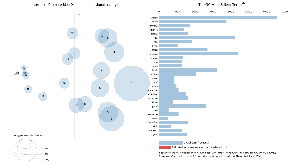
# 4) 문서 별 토픽 분포 보기 - 상위 5개
for i, topic_list in enumerate(ldamodel[corpus]):
    if i==5:
        break
    print(i,'번째 문서 topic 비율: ',topic_list)

# (토픽 번호, 토픽이 해당 문서에서 차지하는 분포도)
0 번째 문서 topic 비율: [(2, 0.42456737), (5, 0.017701633), (6, 0.30507037), (7, 0.11740385), (11, 0.025931243), (14, 0.09783709)]
1 번째 문서 topic 비율: [(4, 0.19281802), (6, 0.56402504), (8, 0.034390826), (16, 0.18770018)]
2 번째 문서 topic 비율: [(2, 0.08864143), (3, 0.037529983), (6, 0.5558445), (10, 0.020978697), (11, 0.063511066), (14, 0.22198538)]
3 번째 문서 topic 비율: [(2, 0.12930709), (6, 0.44330305), (7, 0.06343465), (12, 0.28526807), (17, 0.06693932)]
4 번째 문서 topic 비율: [(1, 0.36722812), (6, 0.53172415), (19, 0.06954694)]BERTopic
- ref : https://wikidocs.net/162076
- !pip install bertopic[visualization]
from bertopic import BERTopicfrom sklearn.datasets import fetch_20newsgroups
docs = fetch_20newsgroups(subset='all', remove=('headers', 'footers', 'quotes'))['data']
print('총 문서의 수 :', len(docs))총 문서의 수 : 18846model = BERTopic(nr_topics = 10)
topics, probabilities = model.fit_transform(docs)print('각 문서의 토픽 번호 리스트 :',len(topics))
print('두번째 문서의 토픽 번호 :', topics[1])각 문서의 토픽 번호 리스트 : 18846
두번째 문서의 토픽 번호 : -1model.get_topic_info()| Topic | Count | Name | |
|---|---|---|---|
| 0 | -1 | 13065 | -1_the_to_of_and |
| 1 | 0 | 1852 | 0_the_to_in_and |
| 2 | 1 | 649 | 1_the_to_of_and |
| 3 | 2 | 512 | 2_the_of_to_in |
| 4 | 3 | 479 | 3_the_car_and_it |
| 5 | 4 | 460 | 4_drive_the_scsi_drives |
| 6 | 5 | 456 | 5_ites_cheek_why_yep |
| 7 | 6 | 441 | 6_for_and_the_to |
| 8 | 7 | 332 | 7_the_to_they_that |
| 9 | 8 | 323 | 8_bike_the_to_and |
| 10 | 9 | 277 | 9_for_and_the_to |
model.get_topic(5)[('ites', 0.7993813137543541),
('cheek', 0.7594094963882347),
('why', 0.6515218145793125),
('yep', 0.6189834540650221),
('huh', 0.5778063889614978),
('ken', 0.5496622938962114),
('luck', 0.5035041768627133),
('forget', 0.49035217536106335),
('art', 0.4862345814829837),
('lets', 0.4355922187643489)]new_doc = docs[0]
print(new_doc)I am sure some bashers of Pens fans are pretty confused about the lack
of any kind of posts about the recent Pens massacre of the Devils. Actually,
I am bit puzzled too and a bit relieved. However, I am going to put an end
to non-PIttsburghers' relief with a bit of praise for the Pens. Man, they
are killing those Devils worse than I thought. Jagr just showed you why
he is much better than his regular season stats. He is also a lot
fo fun to watch in the playoffs. Bowman should let JAgr have a lot of
fun in the next couple of games since the Pens are going to beat the pulp out of Jersey anyway. I was very disappointed not to see the Islanders lose the final
regular season game. PENS RULE!!!topics, probs = model.transform([new_doc])
print('예측한 토픽 번호 :', topics)예측한 토픽 번호 : [0]KeyBERT
import numpy as np
import itertools

from sklearn.feature_extraction.text import CountVectorizer
from sklearn.metrics.pairwise import cosine_similarity
from sentence_transformers import SentenceTransformer
doc = """
Supervised learning is the machine learning task of
learning a function that maps an input to an output based
on example input-output pairs.[1] It infers a function
from labeled training data consisting of a set of
training examples.[2] In supervised learning, each
example is a pair consisting of an input object
(typically a vector) and a desired output value (also
called the supervisory signal). A supervised learning
algorithm analyzes the training data and produces an
inferred function, which can be used for mapping new
examples. An optimal scenario will allow for the algorithm
to correctly determine the class labels for unseen
instances. This requires the learning algorithm to
generalize from the training data to unseen situations
in a 'reasonable' way (see inductive bias).
"""# encoding
# 3개의 단어 묶음인 단어구 추출
n_gram_range = (3, 3)
stop_words = "english"
count = CountVectorizer(ngram_range=n_gram_range, stop_words=stop_words).fit([doc])
candidates = count.get_feature_names_out()
print('trigram 개수 :',len(candidates))
print('trigram 다섯개만 출력 :',candidates[:5])trigram 개수 : 72
trigram 다섯개만 출력 : ['algorithm analyzes training' 'algorithm correctly determine'
'algorithm generalize training' 'allow algorithm correctly'
'analyzes training data']# 키워드 수치화
model = SentenceTransformer('distilbert-base-nli-mean-tokens')
doc_embedding = model.encode([doc])
candidate_embeddings = model.encode(candidates)print(doc_embedding.shape) # 문서별
print(candidate_embeddings.shape) # 단어별 (1, 768)
(72, 768)# 문서와 가장 유사한 키워드 추출
top_n = 5
distances = cosine_similarity(doc_embedding, candidate_embeddings)
keywords = [candidates[index] for index in distances.argsort()[0][-top_n:]]
print(keywords)['algorithm analyzes training', 'learning algorithm generalize', 'learning machine learning', 'learning algorithm analyzes', 'algorithm generalize training']** 키워드 유사도 구하기
- cosine_similarity
- Max Sum Similarity : 데이터 쌍 사이의 최대 합 거리는 데이터 쌍 간의 거리가 최대화되는 데이터 쌍/ 문서와의 후보 유사성을 극대화
- Maximal Marginal Relevance: 텍스트 요약 작업에서 중복을 최소화하고 결과의 다양성을 극대화
def max_sum_sim(doc_embedding, candidate_embeddings, words, top_n, nr_candidates):
    # 문서와 각 키워드들 간의 유사도
    distances = cosine_similarity(doc_embedding, candidate_embeddings)

    # 각 키워드들 간의 유사도
    distances_candidates = cosine_similarity(candidate_embeddings,
                                            candidate_embeddings)

    # 코사인 유사도에 기반하여 키워드들 중 상위 top_n개의 단어를 pick.
    words_idx = list(distances.argsort()[0][-nr_candidates:])
    words_vals = [candidates[index] for index in words_idx]
    distances_candidates = distances_candidates[np.ix_(words_idx, words_idx)]

    # 각 키워드들 중에서 가장 덜 유사한 키워드들간의 조합을 계산
    min_sim = np.inf
    candidate = None
    for combination in itertools.combinations(range(len(words_idx)), top_n):
        sim = sum([distances_candidates[i][j] for i in combination for j in combination if i != j])
        if sim < min_sim:
            candidate = combination
            min_sim = sim

return [words_vals[idx] for idx in candidate]max_sum_sim(doc_embedding, candidate_embeddings, candidates, top_n=5, nr_candidates=10)['requires learning algorithm',
'signal supervised learning',
'learning function maps',
'algorithm analyzes training',
'learning machine learning']def mmr(doc_embedding, candidate_embeddings, words, top_n, diversity):
# 문서와 각 키워드들 간의 유사도가 적혀있는 리스트
word_doc_similarity = cosine_similarity(candidate_embeddings, doc_embedding)
# 각 키워드들 간의 유사도
word_similarity = cosine_similarity(candidate_embeddings)
# 문서와 가장 높은 유사도를 가진 키워드의 인덱스를 추출.
# 만약, 2번 문서가 가장 유사도가 높았다면
# keywords_idx = [2]
keywords_idx = [np.argmax(word_doc_similarity)]
# 가장 높은 유사도를 가진 키워드의 인덱스를 제외한 문서의 인덱스들
# 만약, 2번 문서가 가장 유사도가 높았다면
# ==> candidates_idx = [0, 1, 3, 4, 5, 6, 7, 8, 9, 10 ... 중략 ...]
candidates_idx = [i for i in range(len(words)) if i != keywords_idx[0]]
# 최고의 키워드는 이미 추출했으므로 top_n-1번만큼 아래를 반복.
# ex) top_n = 5라면, 아래의 loop는 4번 반복됨.
for _ in range(top_n - 1):
candidate_similarities = word_doc_similarity[candidates_idx, :]
target_similarities = np.max(word_similarity[candidates_idx][:, keywords_idx], axis=1)
# MMR을 계산
mmr = (1-diversity) * candidate_similarities - diversity * target_similarities.reshape(-1, 1)
mmr_idx = candidates_idx[np.argmax(mmr)]
# keywords & candidates를 업데이트
keywords_idx.append(mmr_idx)
candidates_idx.remove(mmr_idx)
return [words[idx] for idx in keywords_idx]mmr(doc_embedding, candidate_embeddings, candidates, top_n=5, diversity=0.2)['algorithm generalize training',
'supervised learning algorithm',
'learning machine learning',
'learning algorithm analyzes',
'learning algorithm generalize']Reference
- https://sragent.tistory.com/entry/Latent-Semantic-AnalysisLSA
- https://wikidocs.net/24949
- https://bab2min.tistory.com/category/%EA%B7%B8%EB%83%A5%20%EA%B3%B5%EB%B6%80?page=6
- https://bab2min.tistory.com/567?category=673750
- https://ratsgo.github.io/from%20frequency%20to%20semantics/2017/06/01/LDA/
- https://heeya-stupidbutstudying.tistory.com/entry/DL-BERTopic-%EA%B0%9C%EC%9A%94%EC%99%80-%EC%95%8C%EA%B3%A0%EB%A6%AC%EC%A6%98-Topic-modeling-1?category=1018669