0. Summary
- Background
- Word2vec의 한계 : vector space representation learning의 발달에도 아직 regularities가 아직 부족
(Regularity is the quality of being stable and predictable.)
- Word2vec의 한계 : vector space representation learning의 발달에도 아직 regularities가 아직 부족
- Approach
- global log-bilinear regression
- (1) global matrix factorization와 (2) local context window methods의 장점 결합
- training nonzero elements in a word-word co-occurrence matrix
- global log-bilinear regression
- Results
- word analogy task에서 75% (SOTA)
- NER, similarity task 좋은 성능 보임
- Study Keypoints!
- Word2vec과의 차이점
- 학습 구현
1. Introduction
-
기존 방법론의 한계
-
Matrix Factorization (ex: LSA)
- 각 문서에서의 단어의 빈도수를 카운트해서 matrix 만듦. 이를 차원축소해서(SVD) 잠재된 의미 추론.
- (장) 전체적인 통계 정보 고려 (global co-occurrence matrix 사용)
- (단) 단어간의 의미 유추 작업 (analogy task) 성능 떨어짐.
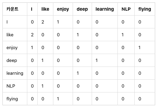
예시
: 전체적으로 enjoy라는 단어가 문장에 자주 나오는 구나~ 그런데 enjoy와 like가 비슷한 맥락의 단어인지는 잘 모르겠네? -
Local context window (ex: skip-gram, word2vec)
- 실제값과 예측값에 대한 오차를 줄이는 학습 방법 사용
- (장) 단어간 의미 유추 작업 성능 LSA보다 뛰어남.
- (단) 윈도우 크기 내 주변 단어만 고려(local context)하기 때문에 전체적인 통계 정보 반영하지 못함
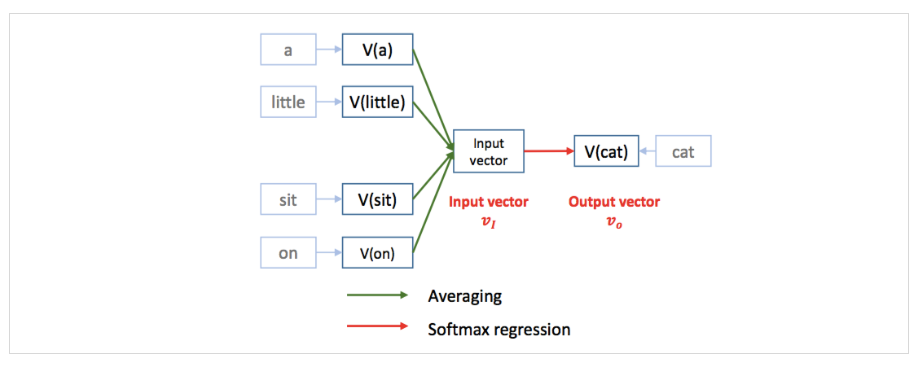
예시
: cat이나 dog이랑 같이 쓰이는 단어가 비슷한 것 보니 둘이 비슷한 embedding vector를 갖겠구나? 하지만, 그 두 단어랑 자주 쓰이는 sit이란 단어는 다른 단어들이랑도 자주 쓰이다보니까 비슷한 embedding vector를 가지고 있지 않네?
-
2. The GloVe Model
-
Loss function
-
Co-occurrence probability
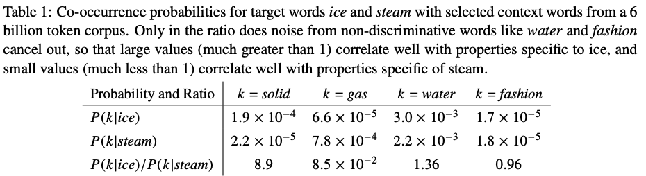
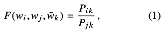
- 단어 간의 동시 등장 확률의 비(ratio)를 벡터 공간에 인코딩해서 단어 간의 의미 추론
- ratio가 big : k 단어는 분자의 단어와 관계가 깊음. (분자 값이 커지니까 = 같이 나타날 확률 높다.)
- ratio가 small : k 단어는 분모의 단어와 관계가 깊음. (분모 값이 커지니까 = 같이 나타날 확률 높다.)
- if, target words : ice & steam 일 때, "solid"는 ice랑 관계가 깊기 때문에 ratio값이 커지고, "gas"는 steam이랑 관계가 깊기 때문에 ratio값이 작아짐.
-
수식
-
Notation
- w_i, w_j : 중심 단어 i, j의 임베딩 벡터
- w_k : 주변 단어 k의 임베딩 벡터
- X_ij : 중심단어 i가 등장했을 때 윈도우 내 주변단어에 j가 등장하는 횟수
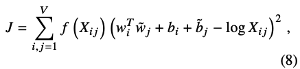
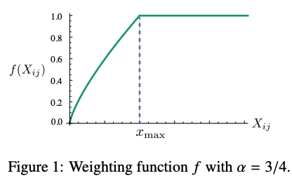
- f(X_ij) : weighting function
-
증명
- ex) i= ice, j= steam, k = solid 일 때 Co-occurrence probability ratio
- 좌변은 벡터, 우변은 스칼라 값이므로 내적을 통해 양변 형태 맞춰준다.
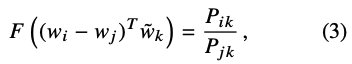
- group homomorphism이란 걸 식에 적용하면 아래와 같이 정리가 된다고함 ^^ (다음부터는 k단어가 j로 재명명)
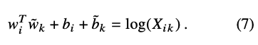
- 최종적으로 i와 k (ice & solid)의 벡터값을 곱한 것이, co-occurrence 의 log 값과 같아지도록 학습. 둘의 동시발생횟수가 높아지면 log값은 커지고, 이에 따라 내적의 곱도 커져야한다. (내적의 곱이 크다 = cosine similarity 높다 = 둘이 비슷하다.)
** 결과적으로는 Word2Vec과 비슷한 학습 결과가 유도되며, Levy & Goldberg에서 이론적으로 word2vec가 glove가 같음을 증명했다고 함.
- Levy, O., & Goldberg, Y. (2014). Neural word embedding as implicit matrix factorization. In Advances in neural information processing systems (pp. 2177-2185).
- ex) i= ice, j= steam, k = solid 일 때 Co-occurrence probability ratio
-
-
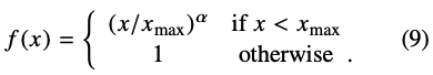
- Weighted error f(x_ij)
- 만약 동시발생율이 너무 작다면 log(X_ij)가 0이 되어버릴 수 있음. 등장 빈도가 낮으면 학습에 전혀 도움이 되지 않을 것이다!
- 그래서! 동시 발생 빈도수가 적은 경우에는 중요도를 낮춰서 학습을 할 수 있도록 한다.
- 동시발생빈도수가 적으면 작은 weight를 곱해주고, 값이 크면 상대적으로 높은 값의 weight를 준다. (a = 3/4)
3. Experiments & Results
-
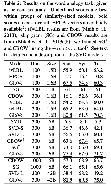
Word analogy
- GloVe가 다른 baseline보다 우수.
- 작은 vector size와 corpora에서도 좋은 성능 보임
-
Word Similarity
- GloVe good
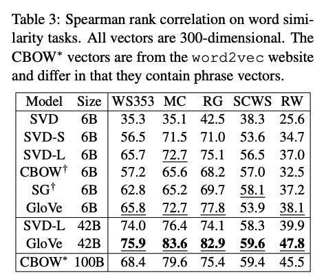
- GloVe good
-
Named Entity Recognition (NER)
- GloVe good
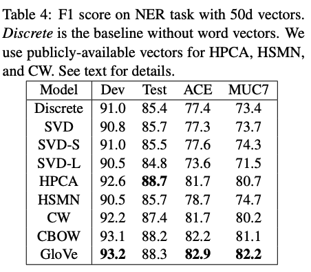
- GloVe good
4. Code Implementation
Contents
- 패키지 사용해서 GloVe 훈련시키기
- Scratch로 GloVe 훈련시키기
- Word2vec과 비교
4-0. 데이터 로드
import re
import urllib.request
import zipfile
from lxml import etree
from nltk.tokenize import word_tokenize, sent_tokenize
# 데이터 다운로드
urllib.request.urlretrieve("https://raw.githubusercontent.com/ukairia777/tensorflow-nlp-tutorial/main/09.%20Word%20Embedding/dataset/ted_en-20160408.xml", filename="ted_en-20160408.xml")
# 전처리
targetXML = open('ted_en-20160408.xml', 'r', encoding='UTF8')
target_text = etree.parse(targetXML)
# xml 파일로부터 <content>와 </content> 사이의 내용만 가져온다.
parse_text = '\n'.join(target_text.xpath('//content/text()'))
# 정규 표현식의 sub 모듈을 통해 content 중간에 등장하는 (Audio), (Laughter) 등의 배경음 부분을 제거.
# 해당 코드는 괄호로 구성된 내용을 제거.
content_text = re.sub(r'\([^)]*\)', '', parse_text)len(content_text) # 너무 많아서 잘라서 사용
> 24062319# 입력 코퍼스에 대해서 NLTK를 이용하여 문장 토큰화를 수행.
sent_text = sent_tokenize(content_text[:1000000])
len(sent_text)
> 10975 # 각 문장에 대해서 구두점을 제거하고, 대문자를 소문자로 변환.
normalized_text = []
for string in sent_text:
tokens = re.sub(r"[^a-z0-9]+", " ", string.lower())
normalized_text.append(tokens)
# 각 문장에 대해서 NLTK를 이용하여 단어 토큰화를 수행.
result = [word_tokenize(sentence) for sentence in normalized_text]print('총 샘플의 개수 : {}'.format(len(result)))
> 총 샘플의 개수 : 10975
# 샘플 3개만 출력
for line in result[:3]:
print(line)
> ['here', 'are', 'two', 'reasons', 'companies', 'fail', 'they', 'only', 'do', 'more', 'of', 'the', 'same', 'or', 'they', 'only', 'do', 'what', 's', 'new']
> ['to', 'me', 'the', 'real', 'real', 'solution', 'to', 'quality', 'growth', 'is', 'figuring', 'out', 'the', 'balance', 'between', 'two', 'activities', 'exploration', 'and', 'exploitation']
> ['both', 'are', 'necessary', 'but', 'it', 'can', 'be', 'too', 'much', 'of', 'a', 'good', 'thing']4-1. Scratch로 GloVe 훈련시키기
- reference : https://www.kaggle.com/datasets/rajat95gupta/practical-ml-implementations-in-python?resource=download
import numpy as np
import matplotlib.pyplot as plt
import nltk
from nltk.corpus import stopwords
import itertools
from collections import Counter
from sklearn.decomposition import PCA
from sklearn.metrics.pairwise import cosine_similarity

nltk.download('brown')
nltk.download('stopwords')
stopwords = stopwords.words('english')

bool_train = True
# info
# number of training epochs
n_epochs = 200
# tolerance
eps = 0.001
# number of sentences to consider
n_sents = 10
# weight embedding size
embedding_size = 100
# learning rate
alpha = 0.1
# AdaGrad parameter
delta = 0.8
# context_window_size
window_size = 5
# top N similar words
topN = 5# 전처리
brown = nltk.corpus.brown
sents = brown.sents()[:n_sents]
print('Processing sentences..\n')
processed_sents = []
for sent in sents:
processed_sents.append([word.lower() for word in sent if word.isalnum() and word not in stopwords])
tokens = list(set(list(itertools.chain(*processed_sents))))
n_tokens = len(tokens)
print('Number of Sentences:', len(sents))
print('Number of Tokens:', n_tokens)Processing sentences..
Number of Sentences: 10
Number of Tokens: 100def get_co_occurences(token, processed_sents, window_size):
"""
window 사이즈만큼 sentence의 앞뒤 간격 확인
"""
co_occurences = []
for sent in processed_sents:
for idx in (np.array(sent)==token).nonzero()[0]:
co_occurences.append(sent[max(0, idx-window_size):min(idx+window_size+1, len(sent))])
co_occurences = list(itertools.chain(*co_occurences))
co_occurence_idxs = list(map(lambda x: token2int[x], co_occurences))
co_occurence_dict = Counter(co_occurence_idxs)
co_occurence_dict = dict(sorted(co_occurence_dict.items()))
return co_occurence_dict
def get_co_occurence_matrix(tokens, processed_sents, window_size):
for token in tokens:
token_idx = token2int[token]
co_occurence_dict = get_co_occurences(token, processed_sents, window_size)
co_occurence_matrix[token_idx, list(co_occurence_dict.keys())] = list(co_occurence_dict.values())
np.fill_diagonal(co_occurence_matrix, 0)
return co_occurence_matrixdef f(X_wc, X_max, alpha):
"""
weighted error
"""
if X_wc<X_max:
return (X_wc/X_max)**alpha
else:
return 1
def loss_fn(weights, bias, co_occurence_matrix, n_tokens, X_max, alpha):
total_cost = 0
for idx_word in range(n_tokens):
for idx_context in range(n_tokens):
w_word = weights[idx_word]
w_context = weights[n_tokens+idx_context]
b_word = bias[idx_word]
b_context = bias[n_tokens+idx_context]
X_wc = co_occurence_matrix[idx_word, idx_context]
total_cost += f(X_wc, X_max, alpha) * (np.dot(w_word.T, w_context) + b_word + b_context - np.log(1 + X_wc))**2
return total_cost
def gradient(weights, bias, co_occurence_matrix, n_tokens, embedding_size, X_max, alpha):
dw = np.zeros((2*n_tokens, embedding_size))
db = np.zeros(2*n_tokens)
# building word vectors
for idx_word in range(n_tokens):
w_word = weights[idx_word]
b_word = bias[idx_word]
for idx_context in range(n_tokens):
w_context = weights[n_tokens+idx_context]
b_context = bias[n_tokens+idx_context]
X_wc = co_occurence_matrix[idx_word, idx_context]
value = f(X_wc, X_max, alpha) * 2 * (np.dot(w_word.T, w_context) + b_word + b_context - np.log(1 + X_wc))
db[idx_word] += value
dw[idx_word] += value * w_context
# building context vectors
for idx_context in range(n_tokens):
w_context = weights[n_tokens + idx_context]
b_context = bias[n_tokens + idx_context]
for idx_word in range(n_tokens):
w_word = weights[idx_word]
b_word = bias[idx_word]
X_wc = co_occurence_matrix[idx_word, idx_context]
value = f(X_wc, X_max, alpha) * 2 * (np.dot(w_word.T, w_context) + b_word + b_context - np.log(1 + X_wc))
db[n_tokens + idx_context] += value
dw[n_tokens + idx_context] += value * w_word
return dw, db
def adagrad(weights_init, bias_init, n_epochs, alpha, eps, delta):
weights = weights_init
bias = bias_init
r1 = np.zeros(weights.shape)
r2 = np.zeros(bias.shape)
X_max = np.max(co_occurence_matrix)
norm_grad_weights = []
norm_grad_bias = []
costs = []
n_iter = 0
cost = 1
convergence = 1
while cost>eps:
dw, db = gradient(weights, bias, co_occurence_matrix, n_tokens, embedding_size, X_max, alpha)
r1+=(dw)**2
r2+=(db)**2
weights -= np.multiply(alpha / (delta + np.sqrt(r1)), dw)
bias -= np.multiply(alpha / (delta + np.sqrt(r2)), db)
cost = loss_fn(weights, bias, co_occurence_matrix, n_tokens, X_max, alpha)
if n_iter%200==0:
print(f'Cost at {n_iter} iterations:', cost.round(3))
norm_grad_weights.append(np.linalg.norm(dw))
norm_grad_bias.append(np.linalg.norm(db))
costs.append(cost)
n_iter += 1
if n_iter>=n_epochs:
convergence = 0
break
if convergence:
print(f'Converged in {len(costs)} epochs..')
else:
print(f'Training complete with {n_epochs} epochs..')
return weights, bias, norm_grad_weights, norm_grad_bias, costsdef plotting(costs, last_n_epochs, norm_grad_weights, norm_grad_bias):
plt.figure(figsize=(20,5))
plt.subplot(131)
plt.plot(costs[-last_n_epochs:], c='k')
plt.title('cost')
plt.xlabel('epochs')
plt.ylabel('value')
plt.subplot(132)
plt.plot(norm_grad_weights[-last_n_epochs:], c='k')
plt.title('norm_weights')
plt.xlabel('epochs')
plt.ylabel('value')
plt.subplot(133)
plt.plot(norm_grad_bias[-last_n_epochs:], c='k')
plt.title('norm_bias')
plt.xlabel('epochs')
plt.ylabel('value')
plt.show()def plotting_word_vectors(weights):
pca = PCA(n_components = 2)
weights = pca.fit_transform(weights[:n_tokens])
explained_var = (100 * sum(pca.explained_variance_)).round(2)
print(f'Variance explained by 2 components: {explained_var}%')
fig, ax = plt.subplots(figsize=(20,10))
for word, x1, x2 in zip(tokens, weights[:,0], weights[:,1]):
ax.annotate(word, (x1, x2))
x_pad = 0.5
y_pad = 1.5
x_axis_min = np.amin(weights, axis=0)[0] - x_pad
x_axis_max = np.amax(weights, axis=0)[0] + x_pad
y_axis_min = np.amin(weights, axis=1)[1] - y_pad
y_axis_max = np.amax(weights, axis=1)[1] + y_pad
plt.xlim(x_axis_min,x_axis_max)
plt.ylim(y_axis_min,y_axis_max)
plt.rcParams["figure.figsize"] = (10,10)
plt.show()if bool_train:
token2int = dict(zip(tokens, range(len(tokens))))
int2token = {v:k for k,v in token2int.items()}
print('Building co-occurence matrix..')
co_occurence_matrix = np.zeros(shape=(len(tokens), len(tokens)), dtype='int')
co_occurence_matrix = get_co_occurence_matrix(tokens, processed_sents, window_size)
print('Co-occurence matrix shape:', co_occurence_matrix.shape)
assert co_occurence_matrix.shape == (n_tokens, n_tokens)
# co-occurence matrix is similar
assert np.all(co_occurence_matrix.T == co_occurence_matrix)
print('\nTraining word vectors..')
weights_init = np.random.random((2 * n_tokens, embedding_size))
bias_init = np.random.random((2 * n_tokens,))
weights, bias, norm_grad_weights, norm_grad_bias, costs = adagrad(weights_init, bias_init, n_epochs, alpha, eps, delta)
# saving weights
#np.save('weights.npy', weights)Building co-occurence matrix..
Co-occurence matrix shape: (100, 100)
Training word vectors..
Cost at 0 iterations: 9475.834
Training complete with 200 epochs..def find_similar_words(csim, token, topN):
token_idx = token2int[token]
closest_words = list(map(lambda x: int2token[x], np.argsort(csim[token_idx])[::-1][:topN]))
return closest_words
# getting cosine similarities between all combinations of word vectors
csim = cosine_similarity(weights[:n_tokens])
# masking diagonal values since they will be most similar
np.fill_diagonal(csim, 0)
token = 'court'
closest_words = find_similar_words(csim, token, topN)
print(f'Similar words to {token}:', closest_words)
# 원래 코드에선 훈련을 4000번 했음. 그때 similar words는 Similar words to court: ['accepted', 'merger', 'recommended', 'presentments', 'charged']
# 확실히 더 많은 훈련이 필요한가봄!Similar words to court: ['follow', 'grand', 'superior', 'operated', 'achieve']print('Plotting learning curves..')
last_n_epochs = 3300
plotting(costs, last_n_epochs, norm_grad_weights, norm_grad_bias)
print('Plotting word vectors..')
plotting_word_vectors(weights)Plotting learning curves..
Plotting word vectors..
Variance explained by 2 components: 29.21%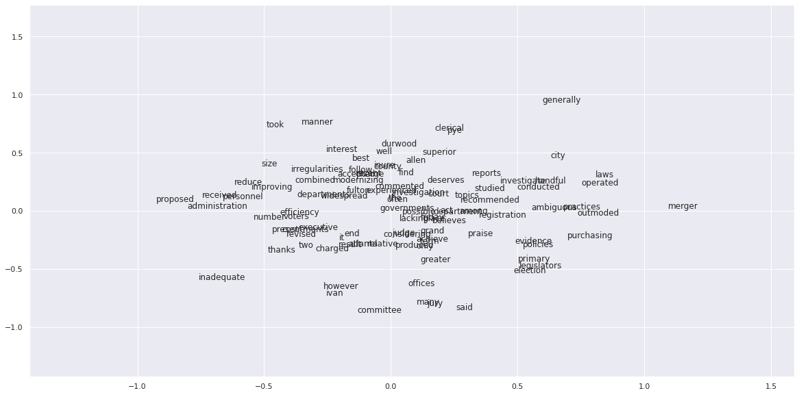
4-2. 패키지 사용해서 GloVe 훈련시키기
- referecne : https://wikidocs.net/22885
! pip install glove_python_binaryfrom glove import Corpus, Glove
corpus = Corpus()
# 훈련 데이터로부터 GloVe에서 사용할 동시 등장 행렬 생성
corpus.fit(result, window=5)
glove = Glove(no_components=100, learning_rate=0.05)
# 학습에 이용할 쓰레드의 개수는 4로 설정, 에포크는 20.
glove.fit(corpus.matrix, epochs=20, no_threads=4, verbose=True)
glove.add_dictionary(corpus.dictionary) # Supply a word-id dictionary to allow similarity queries.print(glove.most_similar("man"))[('great', 0.968211303545362), ('being', 0.9616210663704091), ('long', 0.9527065721465348), ('different', 0.9502125688803607)]4-3. Word2vec과 비교
from gensim.models import Word2Vec
from gensim.models import KeyedVectors

w2v = Word2Vec(sentences=result, vector_size=100, window=5, min_count=5, workers=4, sg=0)
model_result = w2v.wv.most_similar("man")
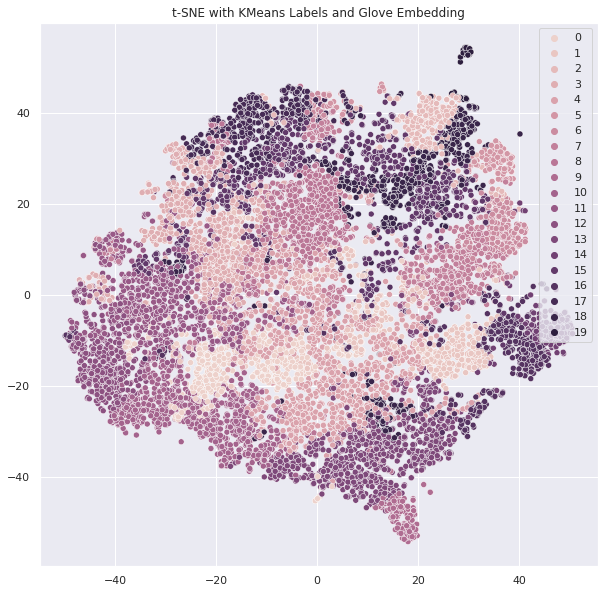
print(model_result)[('week', 0.9982839822769165), ('number', 0.9981682300567627), ('small', 0.9979417324066162), ('written', 0.9978368282318115), ('test', 0.9975178241729736), ('heart', 0.9974570274353027), ('made', 0.9974565505981445), ('special', 0.9974154829978943), ('called', 0.9973793625831604), ('moving', 0.9973017573356628)]시각화
- K-means 알고리즘으로 clustering 후 t-SNE 시각화
- reference : https://jxnjxn.tistory.com/49
# sklearn
from sklearn.cluster import KMeans
from sklearn.manifold import TSNE
# 시각화
import seaborn as sns
import matplotlib.pyplot as plt
def sent2vec_glove(tokens, model, embed_type, embedding_dim=100):
'''문장 token 리스트를 받아서 임베딩 시킨다.'''
size = len(tokens)
matrix = np.zeros((size, embedding_dim))
if embed_type == 'w2v':
word_table = model.wv.key_to_index # glove word_dict
for i, token in enumerate(tokens):
vector = np.array([
model.wv.get_vector(t) for t in token
if t in word_table
])
if vector.size != 0:
final_vector = np.mean(vector, axis=0)
matrix[i] = final_vector
elif embed_type == 'glove':
word_table = model.dictionary # glove word_dict
for i, token in enumerate(tokens):
vector = np.array([
model.word_vectors[model.dictionary[t]] for t in token
if t in word_table
])
if vector.size != 0:
final_vector = np.mean(vector, axis=0)
matrix[i] = final_vector
return matrix# 문장 임베딩 glove
sentence_glove = sent2vec_glove(result, glove, 'glove')
sentence_w2v = sent2vec_glove(result,w2v,'w2v' )# glove clustering
k = 20
kmeans = KMeans(n_clusters=k, random_state=2021)
y_pred = kmeans.fit_predict(sentence_glove)
# tsne
tsne = TSNE(verbose=1, perplexity=100, random_state=2021) # perplexity : 유사정도
X_embedded = tsne.fit_transform(sentence_glove)
print('Embedding shape 확인', X_embedded.shape)
# 시각화
sns.set(rc={'figure.figsize':(10,10)})
# plot
sns.scatterplot(X_embedded[:,0], X_embedded[:,1], hue=y_pred,
legend='full') # kmeans로 예측
plt.title('t-SNE with KMeans Labels and Glove Embedding')
plt.show()
# word2vec도 똑같이 실행!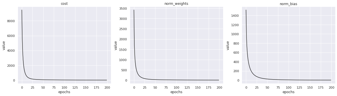
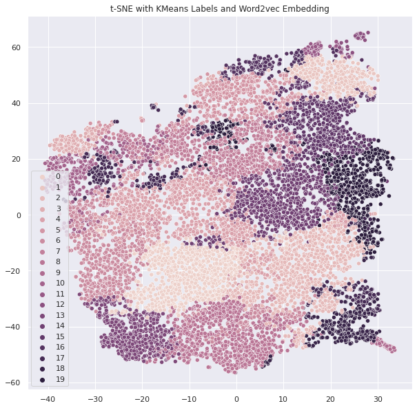
결론 : word2vec, glove 중 좋은걸로 한다!
Reference

왈왈