LSTM

블로그1, 블로그2와 Stanford CS231 lecture를 참조하였습니다.
실험 결과 자료는 여기를 참조했습니다.
블로그

Introduction with RNN

우리는 기존에 시퀀스 데이터를 처리하기 위해 RNN이라는 Network를 고안하였다. 하지만 RNN의 고질적인 문제로 뽑히는 Long-Term-Dependency 문제로 새롭게 만들어진 것이 바로 LSTM이다. 본격적으로 LSTM에 대해 알아보기 이전에, RNN의 구조와 Gradient Vanishing/Exploding 문제를 알아보자.

RNN?

RNN은 기본적으로 순환적인(Recurrent) 구조를 가지고 있다. 이를 그림 오른쪽과 같이 펼쳐서 생각해보자.

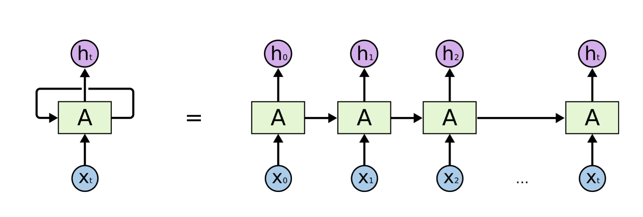
일정한 순서를 가지는 시퀀스 데이터를 각 시점에서 입력받을 때마다 나오는 결과물을 Hidden State라고 할 때, 다음 시점에서는 각 Cell에서 새로운 시퀀스의 데이터와 이전 시점에서의 Hidden State를 학습하여 Hidden State를 갱신한다.
쉽게 이야기하면, 이전 시점까지의 정보를 가지는 Hiddent State와 현재의 입력 $x_t$을 통해 시퀀스 데이터로부터 어떠한 Context vector를 출력하는 형태이다.

Gradient Vanishing/Exploding

RNN은 하지만 입력 데이터의 길이가 길어지면 길어질수록 먼 거리의 데이터가 가지는 정보를 거의 가지지 못하게 된다는 큰 단점이 있다. 이를 Gradient Vanishing/Exploding으로 이야기하는데, '입력 데이터의 정보를 기억한다'는 점과 'Gradient'가 어떠한 관계에서 나온 것인지 살펴보자.

Gradient Vanishing과 관련해서 어느정도 이해하고 있다는 가정으로 진행해보려 한다. Gradient Vanishing 문제와 관련해서 여기에 간략하게 정리해놓았다.

보통의 딥러닝의 경우 Backpropagation에서 Sigmoid를 쓸 수록 Gradient Vanishing 문제가 심화된다는 것을 알고 있었다. 이를 조금이나마 보완하고자 Tanh 함수를 사용하게되었는데, 여전히 RNN에서는 같은 문제가 있었다. 여기서는 Tanh를 Activation Function으로 가정하고 진행하겠다.

RNN Gradient 수식 정리

vanilla RNN 셀 𝑡번째 시점의 히든스테이트 ℎ𝑡는 다음과 정의해보자.($𝑥_𝑡$ : 𝑡번째 시점의 입력, $𝑊_{ℎℎ},𝑊_{𝑥ℎ},𝑏_h$ : 학습 파라메터)

$ℎ_𝑡=tanh(𝑊_{ℎℎ}ℎ_{𝑡−1}+𝑊_{𝑥h}{𝑥_𝑡}+𝑏_ℎ)$

$= tanh(𝑧_𝑡)$

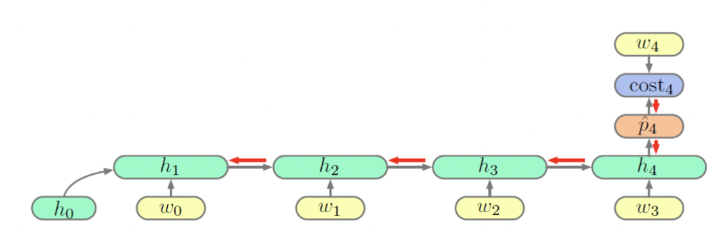
위 그림과 같은 RNN 구조에서 네번째 시점의 손실 $𝑐𝑜𝑠𝑡_4$에 대한 $ℎ_1$의 그래디언트는 체인룰(chain rule)에 의해 아래와 같이 계산할 수 있다.

$\frac{\partial \operatorname{cost}_{4}}{\partial h_{1}}=\frac{\partial \operatorname{cost}_{4}}{\partial \hat{p}_{4}} \frac{\partial \hat{p}_{4}}{\partial h_{4}} \frac{\partial h_{4}}{\partial h_{3}} \frac{\partial h_{3}}{\partial h_{2}} \frac{\partial h_{2}}{\partial h_{1}}$

위 식을 일반화하여 $n$ 번째 시점의 손실 $\operatorname{cost}_{n}$ 에 대한 $h_{1}$ 의 그래디언트는 다음과 같이 표시할 수 있다.

$\frac{\partial \cos t_{n}}{\partial h_{1}}=\frac{\partial \cos t_{n}}{\partial \hat{p}_{n}} \frac{\partial \hat{p}_{n}}{\partial h_{n}}\left(\prod_{t=2}^{n} \frac{\partial h_{t}}{\partial h_{t-1}}\right)$

우리가 이야기하는 RNN의 Gradient문제는 괄호 안의 인자가 계속해서 곱해져 발생하게 된다. 즉, $n$이 커질수록 괄호 안의 값은 계속해서 작아지거나 커질 것이다.

그럼 괄호 안의 인자를 살펴보자.

$h_{t}=\tanh \left(z_{t}\right)$ 이므로 $t$ 번째 히든스테이트에 대한 $t-1$ 번째 히든스테이트의 그래디언트는 체인룰에 의해 다음과 나타낸다.

$\frac{\partial h_{t}}{\partial h_{t-1}}=\frac{\partial h_{t}}{\partial z_{t}} \frac{\partial z_{t}}{\partial h_{t-1}}$

$z_{t}=W_{h h} h_{t-1}+W_{x h} x_{t}+b_{h}$ 이므로 $\partial z_{t} / \partial h_{t-1}$ 은 $W_{h h}$ 이다. norm의 성질에 의해 다음 부등식이 성립한다.

$\left\|\frac{\partial h_{t}}{\partial h_{t-1}}\right\| \leq\left\|\frac{\partial h_{t}}{\partial z_{t}}\right\|\left\|\frac{\partial z_{t}}{\partial h_{t-1}}\right\|=\left\|\frac{\partial h_{t}}{\partial z_{t}}\right\|\left\|W_{h h}\right\|$

RNN 역전파 시 체인룰에 의해 $\partial h_{t} / \partial h_{t-1}$ 을 지속적으로 곱해주어야 한다. 그런데 우리가 살펴봤듯이 $\partial h_{t} / \partial h_{t-1}$ 의 $\mathrm{L} 2 \mathrm{-norm}$은 $W_{h h}$ 의 $\mathrm{L} 2 \mathrm{-norm}$ 크기에 달려 있다. 다시 말해 $W_{h h}$ L2 norm이 1보다 크다면 앞쪽 스텝으로 올수록 그래디언트가 매우 커질 것이며, 1보다 작다면 반대로 매우 작아지게 될 것이다.

물론 Activation Function의 도함수인 $\partial h_{t} / \partial z_{t}$을 계속 곱해주어서 Sigmoid나 Tanh의 경우 Gradient Vanishing문제에 영향을 미친다. 아래는 Activation function별 예측 테스트 결과이다.
ReLU는 Gradient가 1인데도 불구하고 높은 성능을 보여주지 못한다. RNN에서는 그 구조상 $W_{hh}$의 큰 영향으로 인해 기울기 소실 및 증폭 현상이 일어나는 것임을 명심하자.


참고로 L2 norm은 행렬의 Eigenvalue의 최댓값과 같다.

LSTM

위와 같은 Gradient Vanishing 문제를 해결하기 위해 도입된 것이 LSTM이다. 너무 곱하니까 문제가 생기는 것을 확인해서, 더하는 형식을 생각해보는 것이다. 우리는 이를 Cell State라고 부른다.

Cell State

cell state는 기본적으로 어떤 가중치 행렬으로 학습되는 형태가 아니다. hidden state에서 학습된 가중치들로 나온 output들에 대한 선형적 변환으로 정보를 갱신할 뿐이다. 이러한 점이 이전 시점까지의 정보를 잘 유지하고 기억할 수 있게 만들어준다.

하이퍼볼릭탄젠트 안에 있는 내용은 vanilla $\mathrm{RNN}$ 셀과 본질적으로 다르지 않다. $c_{t}$ 를 $c_{t-1}$ 로 미분하는 경우 우변에 $c_{t-1}$ 가 더해졌기 때문에 기본적으로 1을 확보해 그래디언트가 0 으로 죽는 걸 막을 수 있다.
그런데 각 스텝마다 그래디언트가 지속적으로 커진다면 되레 그래디언트 익스플로딩 문제가 발생할 수 있다. 밸런스를 맞춰주기 위해 cell state를 아래와 같이 바꿔보자.

$i_{t}$ 와 $f_{t}$ 는 시그모이드가 취해진 값으로 0, 1사이의 값을 가진다. 각각 직전 시점의 정보, 현 시점의 정보를 얼마나 반영할 지를 결정하게 되고, 다음 히든스테이트를 만들 때도 gate를 둘 수 있다.

$\odot$은 Hadamard product 로, 같은 크기의 행렬 사이에서 같은 위치의 성분끼리 곱하는 방식이다.

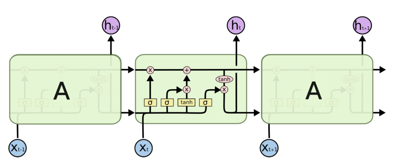
위와 같은 수식을 그림으로 나타낸 것이 아래의 유명한 그림이다.

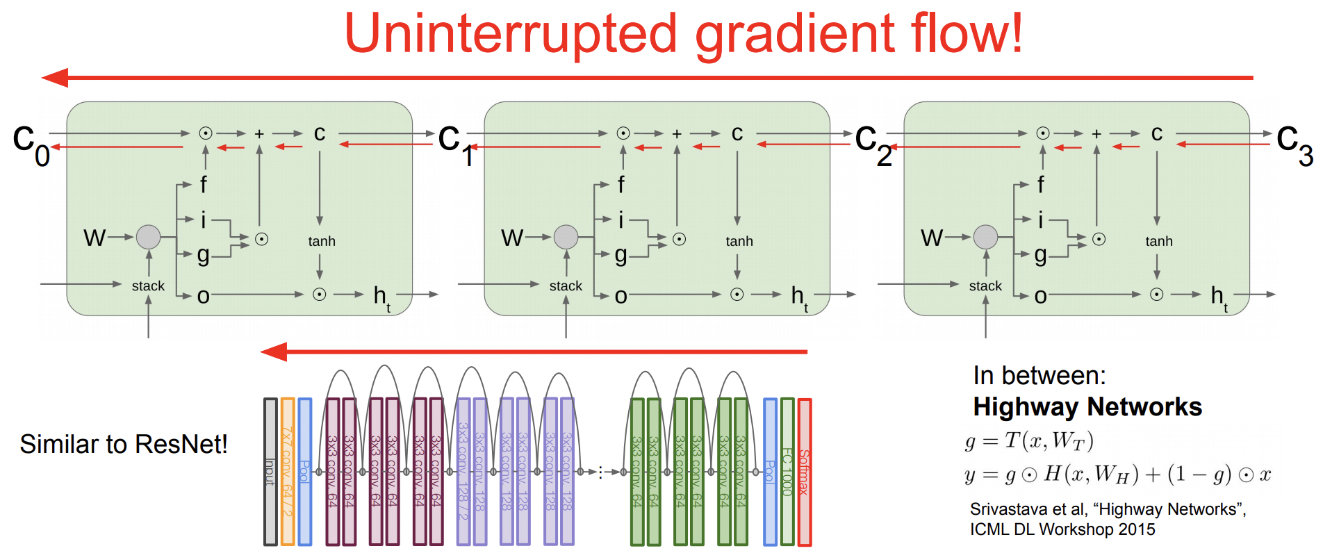
LSTM and ResNet

LSTM은 hidden state 외에 cell state를 가지고 있다. 그리고 이 cell state가 계속 끝까지 흘러가는 형태이다. forget gate가 없는 LSTM이라고 가정하면, 매 time step에 cell state가 Neural Network안에 leak이 되어 hidden state를 업데이트한다. 그 cell state를 보고 computation을 하고 cell state를 additive하게 업데이트한다. 즉 Vanilla RNN이 hidden state를 transformative하게 바꾸는 것에서 차이점이 있다.

그래서 마지막에 Back propagation으로 gradient 업데이트를 할때 이 gradient는 LSTM 구조에서 초기 input 끝까지 흘러들어간다. 그리고 각 f도 나름 gradient를 계산해서 additive하게 더해준다. Karpathy는 이를 Gradient super highway라고 표현했으며, ResNet과 유사하다. 결론적으로 gradient가 죽어버리는 gradient vanshing 문제가 일어나지 않는다.

LSTM and DenseNet

Concatenate
LSTM의 입력에서 이전 시점의 hidden state와 현재 시점의 x데이터를 Concatenation 해주는데, 이는 DenseNet에서 살펴본 적 있었던 방법이다.

Advantage of DenseNet(Concatenate) :
Click here to find more informations
1. Strong Gradient Flow
The error signal can be easily propagated to earlier layers more directly. This is a kind of implicit deep supervision as earlier layers can get direct supervision from the final classification layer.

2. Parameter & Computational Efficiency
For each layer, number of parameters in ResNet is directly proportional to C×C while Number of parameters in DenseNet is directly proportional to l×k×k. Since k<<C, DenseNet has much smaller size than ResNet.

3. More Diversified Features
Since each layer in DenseNet receive all preceding layers as input, more diversified features and tends to have richer patterns.

4. Maintains Low Complexity Features
In DenseNet, classifier uses features of all complexity levels. It tends to give more smooth decision boundaries. It also explains why DenseNet performs well when training data is insufficient.