관련 프로젝트를 마무리하고 그에 관한 정보들을 올린다. 기간이 정해져있어서 많은 분석을 하지 못한 부분이 아쉬웠다. 하지만 본인이 할 수 있는 부분에서는 최대한 했다고 생각한다. 진행하면서 생긴 아이디어들과 자료들은 추후 프로젝트를 통해서 표현해보도록 하겠다.

Game Production Plan Project

PPT와 발표스크립트, 코드파일을 포함한 추가적인 내용은 깃허브 링크를 참조하시길 바랍니다.
깃허브 링크 : https://github.com/colacan100/Game_Production_Plan_Project

1. 데이터 전처리

데이터의 결측치, 표현방식과 단위 통일, 새로운 feature 추가를 위해서 전처리를 진행하였다.

import pandas as pd
import numpy as np
df = pd.read_csv('/vgames2.csv')

df = df.drop(['Unnamed: 0'], axis=1)
# Genre의 Null 값은 분석을 위해 Drop
df = df.dropna()
# Year 전처리
df['Year'] = df['Year'].apply(np.int64)
for i in range(17):
  df.loc[df['Year'] == i, 'Year'] = 2000+i
df.loc[df['Year'] < 100, 'Year'] += 1900

# 데이터가 적은 Year Drop
df_idx1 = df[df['Year']==2017].index
df_idx2 = df[df['Year']==2020].index
df = df.drop(df_idx1)
df = df.drop(df_idx2)

# 지역별 Sales 전처리
df['NA_Sales'] = df['NA_Sales'].replace({'[kK]': '*0.001', '[mM]': '*1'}, regex=True).map(pd.eval).astype(float)
df['EU_Sales'] = df['EU_Sales'].replace({'[kK]': '*0.001', '[mM]': '*1'}, regex=True).map(pd.eval).astype(float)
df['JP_Sales'] = df['JP_Sales'].replace({'[kK]': '*0.001', '[mM]': '*1'}, regex=True).map(pd.eval).astype(float)
df['Other_Sales'] = df['Other_Sales'].replace({'[kK]': '*0.001', '[mM]': '*1'}, regex=True).map(pd.eval).astype(float)

# Sales 합 Column 추가
df['Sales_sum'] = df['NA_Sales']+df['EU_Sales']+df['JP_Sales']+df['Other_Sales']

2-1. 게임 트렌드 분석 (장르)

연도별로 유행하는 게임트렌드가 있을까를 공급의 측면에서 살펴보기 위해 각 연도마다 가장 많이 출시된 장르와 그 출시량을 시각화하였다.

# 그래프를 위한 처리 (라이브러리, 폰트등)
# 아래 코드로 설치 후 런타임 다시 시작
#!apt -qq -y install fonts-nanum > /dev/null
 
import matplotlib.pyplot as plt
import matplotlib.font_manager as fm
 
fontpath = '/usr/share/fonts/truetype/nanum/NanumBarunGothic.ttf'
font = fm.FontProperties(fname=fontpath, size=10)
fm._rebuild()
 
# 그래프에 retina display 적용
%config InlineBackend.figure_format = 'retina'
 
# Colab 의 한글 폰트 설정
plt.rc('font', family='NanumBarunGothic') 

import matplotlib.pyplot as plt
import seaborn as sns

# 연도별 게임의 트렌드가 있을까 (공급)

# 분석을 위한 데이터프레임 만들기
# 연도별 장르 갯수 추출
df_year_genre = df.groupby(['Year', 'Genre']).size().reset_index(name='Count')
# 장르 중 최댓값 추출
year_genre_bool = df_year_genre.groupby(['Year'])['Count'].transform(max) == df_year_genre['Count']
year_max_genre = df_year_genre[year_genre_bool].reset_index(drop=True)
# 중복값 제거
year_max_genre = year_max_genre.drop_duplicates(subset=['Year','Count']).reset_index(drop=True)
year_max_genre.rename(index = {'Count': 'Sales'}, inplace = True)
year_max_genre

# 연도별 공급 트렌드 그래프: 연도별 흐름을 보여주기 위해서 barplot을 이용했다.
import numpy as np, scipy.stats as st
genre = year_max_genre['Genre'].values
plt.figure(figsize=(20,10))

colors = ["#F15F5F"]
sns.set_palette(sns.color_palette(colors))
year_barplot = sns.barplot(x='Year', y='Count',hue='Genre', data=year_max_genre,hue_order=['Action'])
colors = ["#F29661"]
sns.set_palette(sns.color_palette(colors))
year_barplot = sns.barplot(x='Year', y='Count',hue='Genre', data=year_max_genre,hue_order=['Sports'])
colors = ["#F2CB61"]
sns.set_palette(sns.color_palette(colors))
year_barplot = sns.barplot(x='Year', y='Count',hue='Genre', data=year_max_genre,hue_order=['Fighting'])
colors = ["#BCE55C"]
sns.set_palette(sns.color_palette(colors))
year_barplot = sns.barplot(x='Year', y='Count',hue='Genre', data=year_max_genre,hue_order=['Puzzle'])
colors = ["#4374D9"]
sns.set_palette(sns.color_palette(colors))
year_barplot = sns.barplot(x='Year', y='Count',hue='Genre', data=year_max_genre,hue_order=['Platform'])
colors = ["#5CD1E5"]
sns.set_palette(sns.color_palette(colors))
year_barplot = sns.barplot(x='Year', y='Count',hue='Genre', data=year_max_genre,hue_order=['Misc'])
colors = ["#6799FF"]


cnt = 0
for value in year_max_genre['Count']:
    year_barplot.text(x=cnt, y=value + 5, s=str(genre[cnt] + '-' + str(value)),
            color='black', size=8, rotation=90, ha='center')
    cnt+=1
plt.xticks(rotation=90, fontsize=12)
plt.yticks(fontsize=12)

plt.title('연도별 공급 트렌드 그래프')
plt.xlabel('연도')
plt.ylabel('최대 공급 장르의 출시량')
plt.show()
# 공급 부분에서 최근 트렌드는 Action 장르임을 알 수 있다.

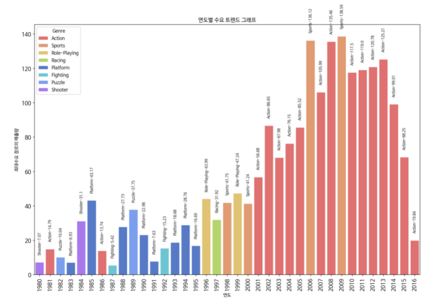
연도별로 유행하는 게임트렌드가 있을까를 수요의 측면에서 살펴보기 위해 각 연도마다 가장 많이 팔린 장르와 그 매출량을 시각화하였다.

# 연도별 게임의 트렌드가 있을까 (수요)

# 연도별 장르 총매출 추출
year_max_sales = df.groupby(['Year', 'Genre'])['Sales_sum'].sum().reset_index()
# 장르 중 최댓값 추출
year_sales_bool = year_max_sales.groupby(['Year'])['Sales_sum'].transform(max) == year_max_sales['Sales_sum']
year_max_sales = year_max_sales[year_sales_bool].reset_index(drop=True)
year_max_sales

# 연도별 수요 트렌드 그래프: 연도별 흐름을 보여주기 위해서 barplot을 이용했다.
genre = year_max_sales['Genre'].values
plt.figure(figsize=(15,10))

colors = ["#F15F5F"]
sns.set_palette(sns.color_palette(colors))
year_barplot = sns.barplot(x='Year', y='Sales_sum',hue='Genre', data=year_max_sales,hue_order=['Action'])
colors = ["#F29661"]
sns.set_palette(sns.color_palette(colors))
year_barplot = sns.barplot(x='Year', y='Sales_sum',hue='Genre', data=year_max_sales,hue_order=['Sports'])
colors = ["#F2CB61"]
sns.set_palette(sns.color_palette(colors))
year_barplot = sns.barplot(x='Year', y='Sales_sum',hue='Genre', data=year_max_sales,hue_order=['Role-Playing'])
colors = ["#BCE55C"]
sns.set_palette(sns.color_palette(colors))
year_barplot = sns.barplot(x='Year', y='Sales_sum',hue='Genre', data=year_max_sales,hue_order=['Racing'])
colors = ["#4374D9"]
sns.set_palette(sns.color_palette(colors))
year_barplot = sns.barplot(x='Year', y='Sales_sum',hue='Genre', data=year_max_sales,hue_order=['Platform'])
colors = ["#5CD1E5"]
sns.set_palette(sns.color_palette(colors))
year_barplot = sns.barplot(x='Year', y='Sales_sum',hue='Genre', data=year_max_sales,hue_order=['Fighting'])
colors = ["#6799FF"]
sns.set_palette(sns.color_palette(colors))
year_barplot = sns.barplot(x='Year', y='Sales_sum',hue='Genre', data=year_max_sales,hue_order=['Puzzle'])
colors = ["#A566FF"]
sns.set_palette(sns.color_palette(colors))
year_barplot = sns.barplot(x='Year', y='Sales_sum',hue='Genre', data=year_max_sales,hue_order=['Shooter'])


cnt = 0
for value in year_max_sales['Sales_sum']:
    year_barplot.text(x=cnt, y=value + 5, s=str(genre[cnt] + '-' + str(round(value,2))),
            color='black', size=8, rotation=90, ha='center')
    cnt+=1
plt.xticks(rotation=90, fontsize=12)
plt.yticks(fontsize=12)
plt.title('연도별 수요 트렌드 그래프')
plt.xlabel('연도')
plt.ylabel('최대수요 장르의 매출량')
plt.show()
# 수요 부분에서 최근 트렌드는 Action 장르임을 알 수 있다.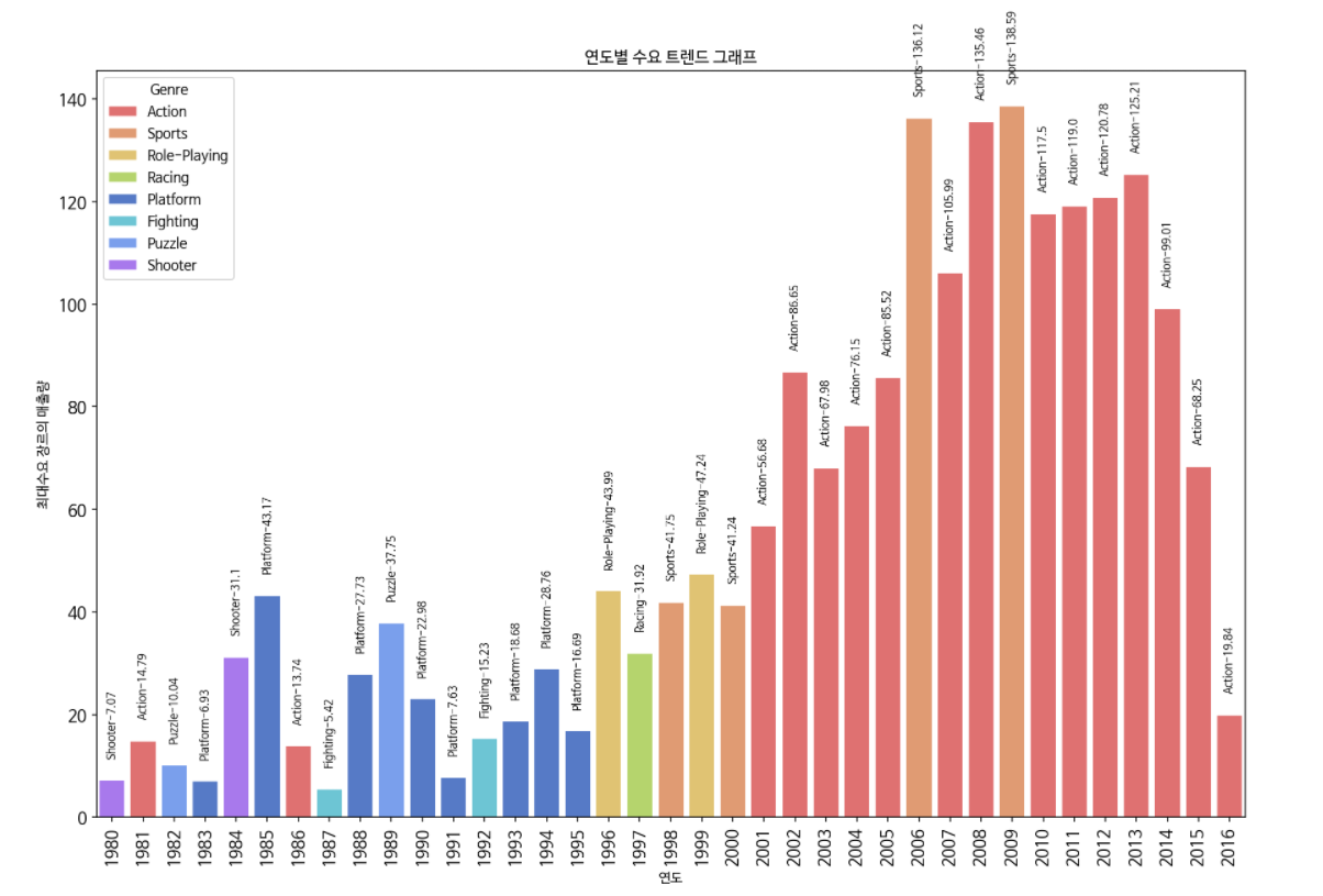

따라서 수요와 공급의 측면에서 연도별 장르의 트렌드가 변화한다는 것을 알 수 있다.

2-2. 게임 트렌드 분석 (플랫폼)

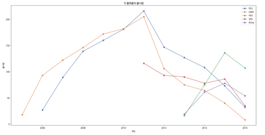
시기에 따라 플랫폼 버전의 변화가 일어날 수 있기에 연도별 각 플랫폼의 출시량을 시각화하였다.

sns.set_palette('deep')

# 연도별 플랫폼 출시 비율 그래프 형태 (꺾은선)
plt.figure(figsize=(20, 10))

# 격자 여백 설정
plt.subplots_adjust(wspace = 0.2, hspace = 0.5)

PS3_filter = df.Platform == 'PS3' # 조건식 작성
df_PS3 = df.loc[PS3_filter]
df_PS3 = df_PS3.groupby(['Year', 'Platform']).size().reset_index(name='Count')
plt.plot(df_PS3['Year'], df_PS3['Count'],marker='o',label = 'PS3')

X360_filter = df.Platform == 'X360' # 조건식 작성
df_X360 = df.loc[X360_filter]
df_X360 = df_X360.groupby(['Year', 'Platform']).size().reset_index(name='Count')
plt.plot(df_X360['Year'], df_X360['Count'],marker='o',label = 'X360')

PS4_filter = df.Platform == 'PS4' # 조건식 작성
df_PS4 = df.loc[PS4_filter]
df_PS4 = df_PS4.groupby(['Year', 'Platform']).size().reset_index(name='Count')
plt.plot(df_PS4['Year'], df_PS4['Count'],marker='o',label = 'PS4')

DS3_filter = df.Platform == '3DS' # 조건식 작성
df_3DS = df.loc[DS3_filter]
df_3DS = df_3DS.groupby(['Year', 'Platform']).size().reset_index(name='Count')
plt.plot(df_3DS['Year'], df_3DS['Count'],marker='o',label = '3DS')

XOne_filter = df.Platform == 'XOne' # 조건식 작성
df_XOne = df.loc[XOne_filter]
df_XOne = df_XOne.groupby(['Year', 'Platform']).size().reset_index(name='Count')
plt.plot(df_XOne['Year'], df_XOne['Count'],marker='o',label = 'XOne')
plt.legend()

plt.title('각 플랫폼의 출시량')
plt.xlabel('연도')
plt.ylabel('출시량')
plt.show()

# X360과 PS3의 경우 콘솔 시장의 변화로 인해 수가 줄어들고 있다.
# 따라서 PS4를 Platform으로 채택한다.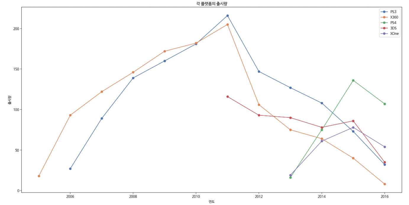

따라서 시기에 따라 플랫폼의 흐름도 변화한다는 것을 알 수 있다.

2-3. 게임 트렌드 분석 (지역)

지역에 따라 선호하는 게임 장르가 다를까에 대해서 분석하기 위해 지역별로 선호장르의 퍼센티지를 Pie 그래프로 나타내었다.

# 분석을 위한 데이터프레임 만들기
locate_Genre_NA = df.groupby(['Genre'])['NA_Sales'].sum()
locate_Genre_EU = df.groupby(['Genre'])['EU_Sales'].sum()
locate_Genre_JP = df.groupby(['Genre'])['JP_Sales'].sum()
locate_Genre_Other = df.groupby(['Genre'])['Other_Sales'].sum()
locate_Genre = pd.DataFrame()
locate_Genre = locate_Genre.append(locate_Genre_NA)
locate_Genre = locate_Genre.append(locate_Genre_EU)
locate_Genre = locate_Genre.append(locate_Genre_JP)
locate_Genre = locate_Genre.append(locate_Genre_Other)
locate_Genre = locate_Genre.T
locate_Genre

pie_locate = locate_Genre.T
pie_label = pie_locate.columns.values.tolist()
plt.figure(figsize=(8, 8))
plt.pie(pie_locate.loc['NA_Sales'], labels=pie_label, autopct='%.1f%%')
plt.title('북미 지역의 선호장르')

plt.figure(figsize=(8, 8))
plt.pie(pie_locate.loc['EU_Sales'], labels=pie_label, autopct='%.1f%%')
plt.title('유럽 지역의 선호장르')

plt.figure(figsize=(8, 8))
plt.pie(pie_locate.loc['JP_Sales'], labels=pie_label, autopct='%.1f%%')
plt.title('일본 지역의 선호장르')

plt.figure(figsize=(8, 8))
plt.pie(pie_locate.loc['Other_Sales'], labels=pie_label, autopct='%.1f%%')
plt.title('그 외 지역의 선호장르')

plt.show()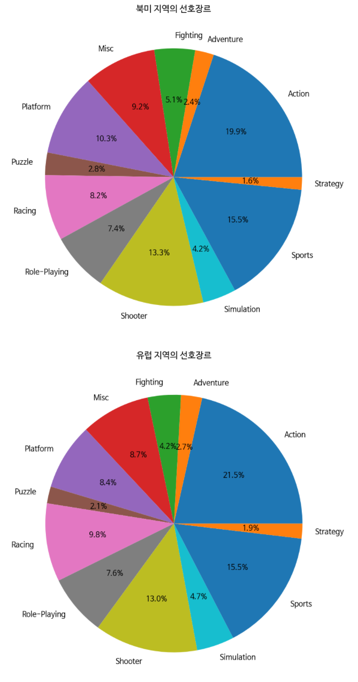

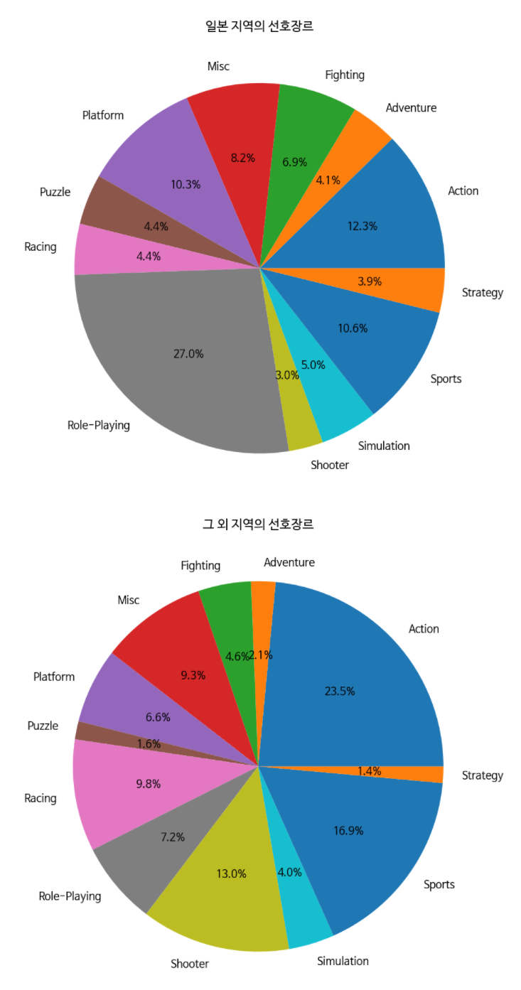
하지만 Pie 그래프로 완벽하게 트렌드를 분석하는 것은 무리가 있다고 판단. 카이제곱 검정을 이용하여 신뢰성을 높이기로 하였다.

from scipy.stats import chi2_contingency
# 카이제곱 검정으로 판단
# 독립변수 : 장르
# 종속변수 : 국가별 판매량
# 귀무가설 : 비율 차이가 없다. (=지역마다 선호하는 장르가 같다.)
chi2_val, p, dof, expected= chi2_contingency(locate_Genre, correction=False)
if(p<0.05) : 
    print('p value:', p,"\n"+'귀무가설을 기각한다. 지역마다 선호하는 장르가 다르다.')
else :
    print('p value:', p,"\n"+'귀무가설을 기각하지 못한다. 지역마다 선호하는 장르가 같다.')

# 일본을 제외한 경우
locate_Genre2 = locate_Genre.drop(['JP_Sales'], axis=1)
chi2_val, p, dof, expected= chi2_contingency(locate_Genre2, correction=False)
if(p<0.05) : 
    print('일본을 제외한 p value:', p,"\n"+'귀무가설을 기각한다. 일본을 제외한 지역마다 선호하는 장르가 다르다.')
else :
    print('p value:', p,"\n"+'귀무가설을 기각하지 못한다. 일본을 제외한 지역마다 선호하는 장르가 같다.')

// 출력결과 //
p value: 9.964279787302075e-123
귀무가설을 기각한다. 지역마다 선호하는 장르가 다르다.
일본을 제외한 p value: 0.024080297712670003
귀무가설을 기각한다. 일본을 제외한 지역마다 선호하는 장르가 다르다.

따라서 지역마다 선호하는 장르가 다르다고 판단했다.

2-4. 게임 트렌드 분석 (출고량 높은 게임)

출고량이 높은 게임의 특성을 확인하기 위해서 최근 10년간의 매출량 Top100을 선정하여 시각화를 진행하였다.

# 출고량이 높은 게임에 대한 분석 및 시각화 프로세스
# 주제에 맞게끔 최근 10년간 판매량 Top 100을 선정
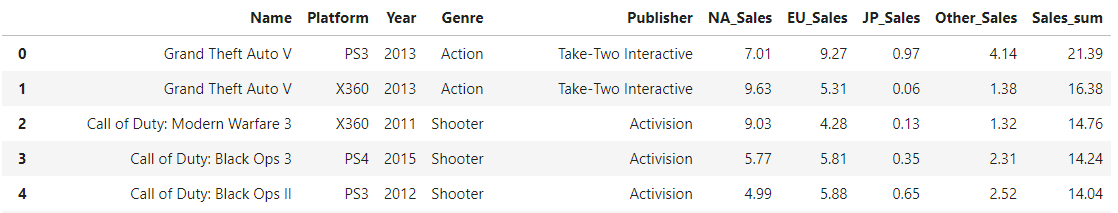
sales_top100 = df[df.Year > 2010].sort_values(by='Sales_sum' ,ascending=False)
sales_top100 = sales_top100.head(100).reset_index(drop=True)
sales_top100

매출량 Top 100의 플랫폼별 매출량 그래프

# top100 Platform 그래프
top100_platform = sales_top100.groupby(['Platform'])['Sales_sum'].sum().reset_index()
platform = top100_platform['Platform'].values
plt.figure(figsize=(10, 10))
top100_platform_sales = sns.barplot(x ='Sales_sum', y='Platform', data=top100_platform)
cnt = 0
for value in top100_platform['Sales_sum']:
    top100_platform_sales.text(x=value + 5, y=cnt, s=str(round(value,2)),
            color='black', size=10)
    cnt+=1
plt.title('매출량 Top 100의 플랫폼별 매출량 (최근 10년)')
plt.xlabel('매출량')
plt.ylabel('플랫폼')
plt.show()
# 최근 10년간 출고량이 많았던 플랫폼은 PS3,PS4,X360이다.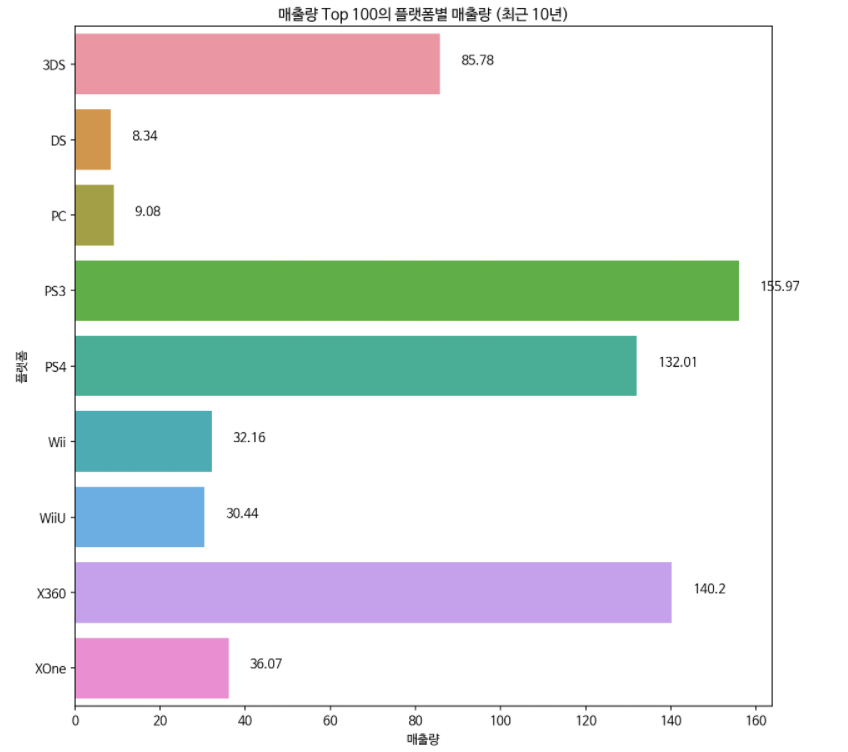

매출량 Top 100의 장르별 매출량 그래프

# top100 Genre 그래프
top100_genre = sales_top100.groupby(['Genre'])['Sales_sum'].sum().reset_index()
genre = top100_genre['Genre'].values
plt.figure(figsize=(10, 10))
top100_genre_sales = sns.barplot(x ='Sales_sum', y='Genre', data=top100_genre)
cnt = 0
for value in top100_genre['Sales_sum']:
    top100_genre_sales.text(x=value + 5, y=cnt, s=str(round(value,2)),
            color='black', size=10)
    cnt+=1
plt.title('매출량 Top 100의 장르별 매출량 (최근 10년)')
plt.xlabel('매출량')
plt.ylabel('장르')
plt.show()
# 최근 10년간 출고량이 많았던 장르는 Shooter,Action,Sports 이다.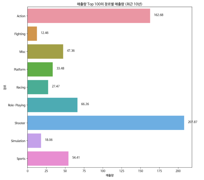

매출량 Top 100의 회사별 매출량 그래프

# top100 Publisher 그래프
top100_publisher = sales_top100.groupby(['Publisher'])['Sales_sum'].sum().reset_index()
publisher = top100_publisher['Publisher'].values
plt.figure(figsize=(10, 10))
top100_publisher_sales = sns.barplot(x ='Sales_sum', y='Publisher', data=top100_publisher)
cnt = 0
for value in top100_publisher['Sales_sum']:
    top100_publisher_sales.text(x=value + 5, y=cnt, s=str(round(value,2)),
            color='black', size=10)
    cnt+=1
plt.title('매출량 Top 100의 회사별 매출량 (최근 10년)')
plt.xlabel('매출량')
plt.ylabel('회사')
plt.show()
# 최근 10년간 출고량이 많았던 회사는 Activision,Nintendo,Electronic Arts 이다.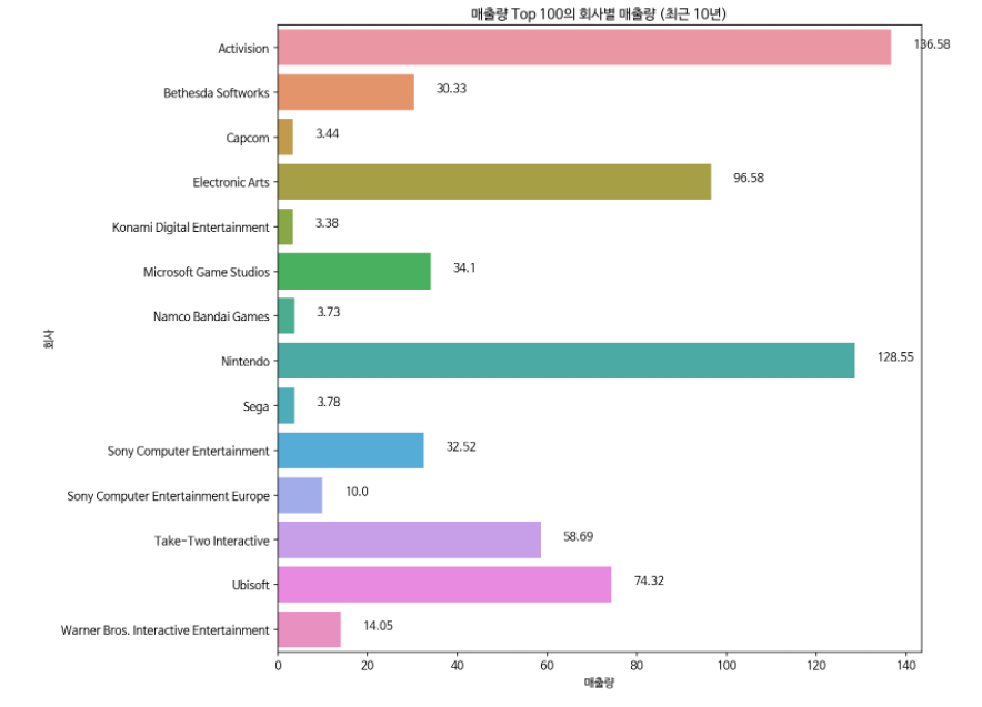

전체 게임 분석과 비교하여 트렌드가 다른 것을 볼 수 있다.

이유는 GTA,Call of Duty와 같은 시리즈물의 영향으로 결과값이 영향을 받았다고 생각한다.
따라서 전체 데이터를 대상으로 선택과정을 진행할 것이다. (출고량이 높은 데이터를 제외할까도 생각해보았지만 시리즈물 또한 트렌드의 일부라고 판단하여 기각하였다.)

3-1. 설계할 게임 선택 (장르)
최근 10년 동안 어떤 장르의 공급 수요가 높은지 시각화하였다. (2-1. 게임 트렌드 분석 (장르)의 코드와 동일하다.)


최근 10년동안 Action장르의 공급,수요가 높으므로 장르는 Action으로 선택하였다.

3-2. 설계할 게임 선택 (플랫폼)
최근 10년 동안 Action 장르에서 어떤 플랫폼의 매출량이 가장 높은지 시각화하였다.

Genre_filter = (df.Genre == 'Action') & (df.Year > 2010) # 조건식 작성
df_action = df.loc[Genre_filter].reset_index(drop = True)
df_action

df_action_platform = df_action.groupby(['Platform'])['Sales_sum'].sum().reset_index()
platform = df_action_platform['Platform'].values
plt.figure(figsize=(10, 10))
df_action_platform_sales = sns.barplot(x ='Sales_sum', y='Platform', data=df_action_platform)
cnt = 0
for value in df_action_platform['Sales_sum']:
    df_action_platform_sales.text(x=value + 5, y=cnt, s=str(round(value,2)),
            color='black', size=10)
    cnt+=1
plt.title('Action게임의 플랫폼별 매출량 (최근 10년)')
plt.xlabel('매출량')
plt.ylabel('플랫폼')
plt.show()

또한, 버전의 변화로 인해 출시량이 급격하게 줄어든 플랫폼을 파악하여 제거하기 위해 최근 10년 동안 플랫폼의 출시량을 살펴보았다. (2-2. 게임 트렌드 분석 (플랫폼)의 코드와 동일하다.)

X360과 PS3의 경우 콘솔 시장의 변화로 인해 수가 줄어들고 있다. 따라서 이 둘을 제외하고 최대 매출량을 가진 PS4를 플랫폼으로 채택하였다.

3-3. 설계할 게임 선택 (지역)

Action장르와 PS4의 플랫폼의 게임이 어느지역에서 가장 큰 매출을 올렸는지 파악한다.

Platform_filter = (df_action.Platform == 'PS4') # 조건식 작성
df_action_ps4 = df_action.loc[Platform_filter].reset_index(drop = True)
df_action_ps4

plt.figure(figsize=(10,10))
locate_NA = df_action_ps4['NA_Sales'].sum()
locate_EU = df_action_ps4['EU_Sales'].sum()
locate_JP = df_action_ps4['JP_Sales'].sum()
locate_Other = df_action_ps4['Other_Sales'].sum()
locate_group = pd.DataFrame({'locate':['NA','EU','JP','Other'],'Sales':[locate_NA, locate_EU,locate_JP,locate_Other]})
locate_barplot = sns.barplot(x='locate', y='Sales',data=locate_group)
Sales = locate_group['Sales'].values
cnt = 0
for value in locate_group['Sales']:
    locate_barplot.text(x=cnt, y=value+0.5, s=str(str(round(value,2))),
            color='black', size=10, ha='center')
    cnt+=1
plt.title('Action게임(PS4)에서 지역별 매출량 (최근 10년)')
plt.xlabel('지역')
plt.ylabel('매출량')
plt.show()
# EU를 대상으로한 게임을 설계한다.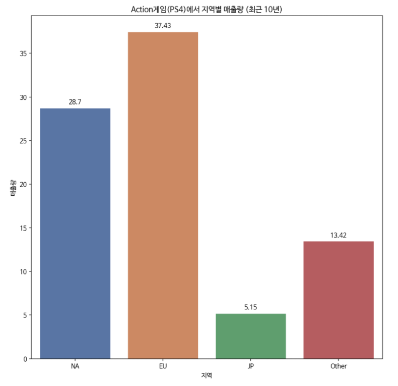

EU지역의 매출량이 가장 높으므로 EU지역을 대상으로한 게임을 설계한다.

3-4. 설계할 게임 선택 (회사)

모티브로할 회사를 결정하기 위해서 위의 조건을 다 만족하는 회사의 매출량을 시각화하였다.

# 연도별 장르 갯수 추출
df_action_ps4_pub = df_action_ps4.groupby(['Publisher'])['EU_Sales'].sum().reset_index()
plt.figure(figsize=(10, 10))
res_barplot = sns.barplot(x='EU_Sales', y='Publisher',data=df_action_ps4_pub)
plt.title('EU지역에서 Action게임(PS4)의 회사별 매출량 (최근 10년)')
plt.xlabel('EU지역 매출량')
plt.ylabel('회사')
plt.show()
# Ubisoft를 모티브로 하겠다.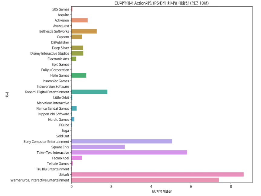

Ubisoft가 가장 매출량이 높으므로 Ubisoft를 모티브로한 게임을 설계한다.

4. 결론
Action 장르로 PS4 플랫폼에서 EU지역을 대상으로 Ubisoft회사를 모티브로 하여 게임을 설계하는 것이 신생회사가 최소의 투자로 최대의 이익을 얻을 수 있는 방법이다.