[CS224N] Lecture 5 - Recurrent Neural networks (RNNs)

🔗 Transition based dependency parsers

• Efficient linear time method for giving the syntatic structure of natural language text
• Neural net이 나오기 전까지는 꽤 잘 작동하는 모델이었다.
• 단점
  • indicator features로 수행했다.

🔗 Problems of indicator features

1. feature들이 sparse하다.
2. feature들이 incomplete하다.

• Training data에서 어떤 words와 configuration이 나타났는지에 따라서 특정 feature들은 존재하고 다른 특정 feature들은 존재하지 않는다. 왜냐하면 training data에서 이 word는 verb 전에 나타났고, 다른 이 word는 verb 전에 절대 안나타났을 수 있기 때문이다.

3. ⭐️ Symbolic dependency parser에서는 이 feature들을 다 계산하는 것이 pretty expensive하다.

• Parsing time의 95%를 feature computation(모든 configuration에서의 모든 feature들을 계산)에 소비하였다.

➡️ Dense and compact feature representation을 학습하자!

A neural dependency parser

[Chen and Manning 2014]

🔗 First win: Distributed Representations

• 각 word를 d-dimensional dense vector(i.e., word embedding)로 표현하였다.
  • 그래서 특정 configuration에서 보지 못한 word여도, configuration에서 비슷한 words를 보았었기 때문에 어떤 것인지 알 수 있었다.
• Part-of-speech tags (POS)와 dependency labels도 d-dimensional vectors(distributed representations)로 표현하였다.
  • 작은 discrete sets도 많은 semantical similarities를 나타낸다.

🔗 Extracting Tokens & vecotr representations from configuration

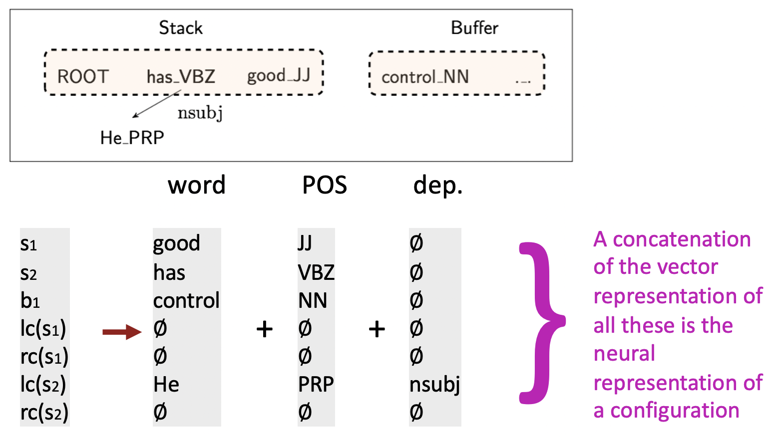
• Symbolic dependency parser와 같은 configuration을 가진다. Stack과 buffer가 있고 arcs를 build한다.
• 이 configuration의 element들을 가져다가 각각의 embedding(word embedding & pos embedding)을 보고 모두를 concatenate한다. 이것이 configuration의 neural representation이 된다.

🔗 Second win: Deep Learning classifiers are non-linear classifiers

• Traditional ML classifiers는 오직 linear decision boundaries만 준다. 그래서 task가 복잡할 때는 효과적이지 않다.
• Neural networks는 non-linear decision boundaries를 제공하기 때문에 훨씬 더 복잡한 function도 학습할 수 있다. 강력하다.
  
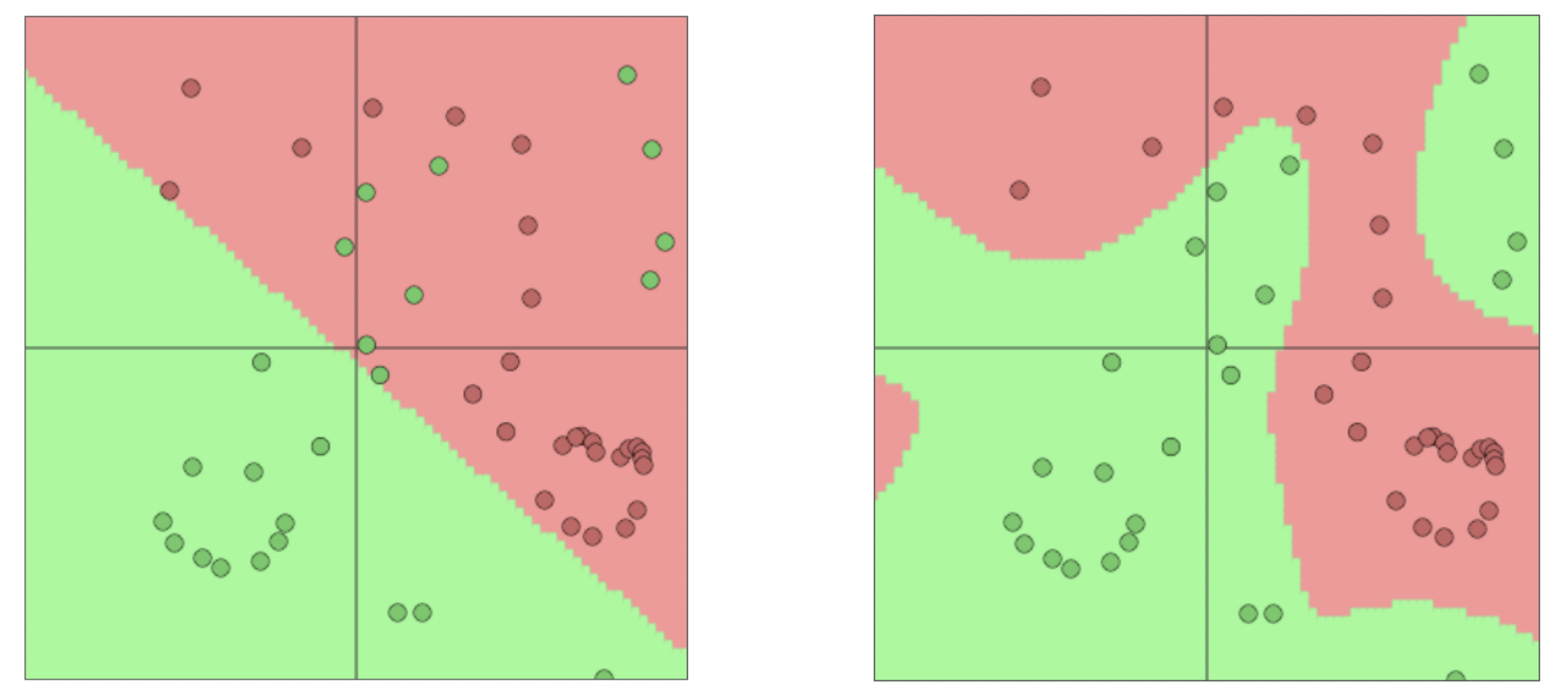
  • 실제로는 original space를 non-linear하게 만들고, neural network의 top에서 softmax로 linear classification을 한다.
  • Neural networ는 space를 warp하여 representation of data points를 옮긴다. 그렇게 하여 결국 Linear classifier로 classification되도록 한다.

🔗 Neural Dependency Parser Model Architecture

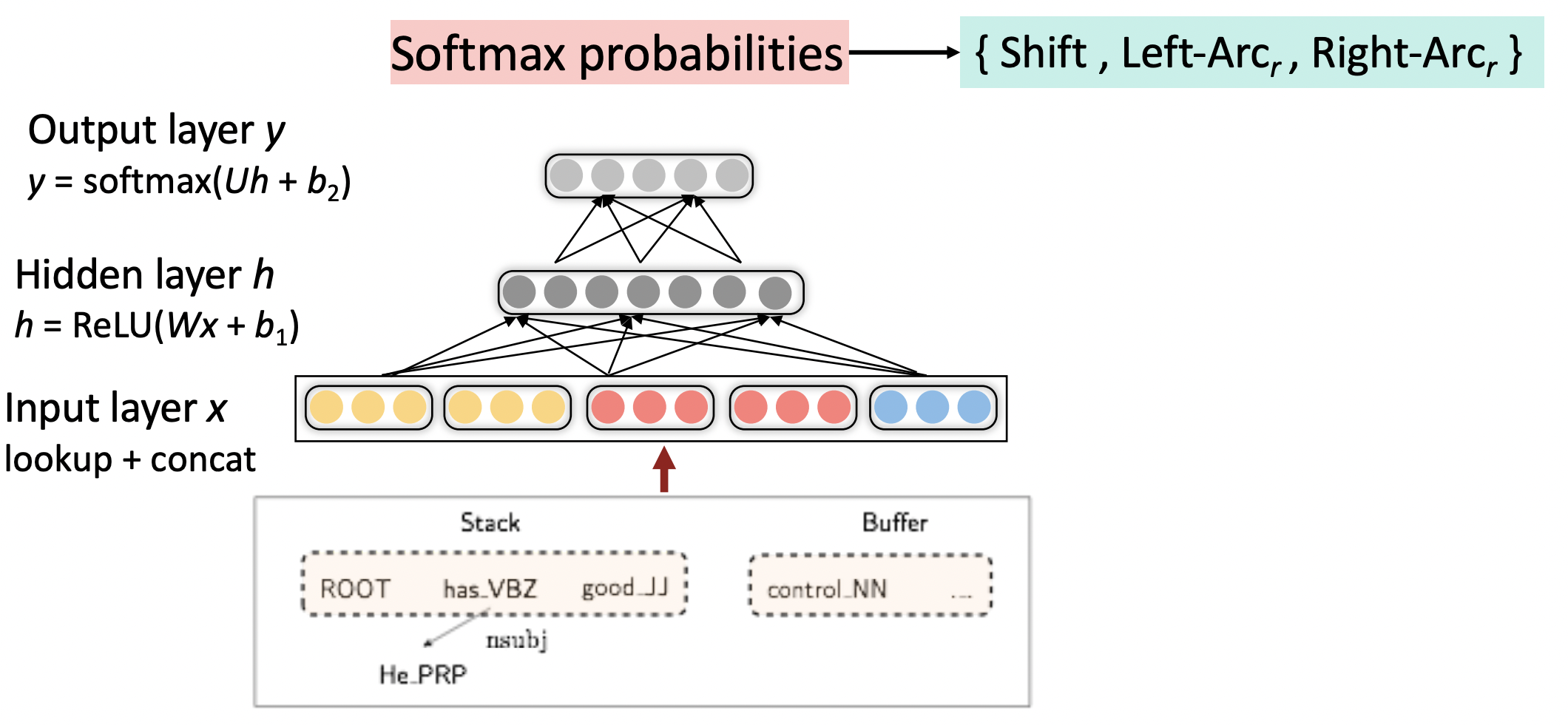
• Transition based dependency parser configuration을 기반으로 input layer embedding을 만든다.
  • Human language를 다룰 때 우리에게 실제로 있는 것은 word와 POS에 대한 one-hot vector이므로 lookup process(one hot feature를 dense input layer로 convert하기 위해 matrix multiply)를 한다.

➡️ 이러한 Dense representations와 non-linear classifier를 통해 accuracy와 speed 측면 둘다에서 다른 greedy parser들을 능가하였다.

Graph-based dependency parsers

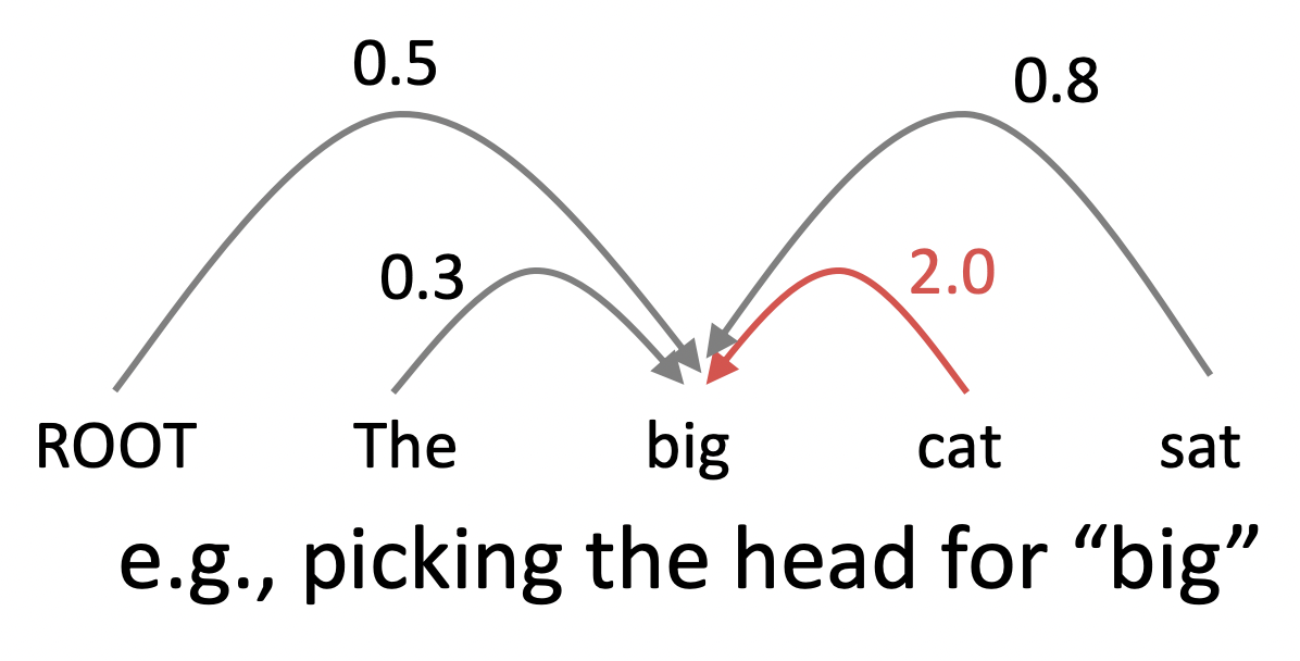
• 각 word마다 모든 가능한 dependency(choice of head)의 score를 계산하여 best one을 선택한다.
• 첫번째 approximation은, 각각의 단어에 대해 가장 dependent로 보이는 word의 dependent인 word를 선택하려고 할 것이다. 우리는 하나의 ROOT를 가진 tree를 얻고 싶은 제약이 있기 때문에 서로 다른 dependencies의 가능성에 대한 score를 사용하는 MST algorithm을 사용한다.

➡️ 성능은 좋지만 simple neural transition-based parsers보다 느리다. 왜냐하면 n^2의 가능한 dependencies가 있기 때문에 linear time에 수행하지 못해 많은 양의 text를 parse하는 것이 오래 걸린다.

🔗 Regularization

• Classic view

  • 많은 수의 feature들이 있을 때 overfitting을 막기 위해 regularization을 수행한다.

• 요즘 view

  • Big neural network를 train하면 항상 training data에 overfitting된다. 매우 overfitting된다. 하지만 train data에 overfitting되는 것은 문제가 아니다. 많은 경우, neural network가 엄청 많은 parameter가 있기 때문에 training data에 대한 error가 0이 될 때까지 계속 train할 수 있다.
  • 그럼에도 불구하고 regularization을 하는 이유는, 모델이 regularization이 잘되면 generalize가 잘 되고 independent test data에 대한 예측을 잘 수행한다.

• L2 Regularization
  

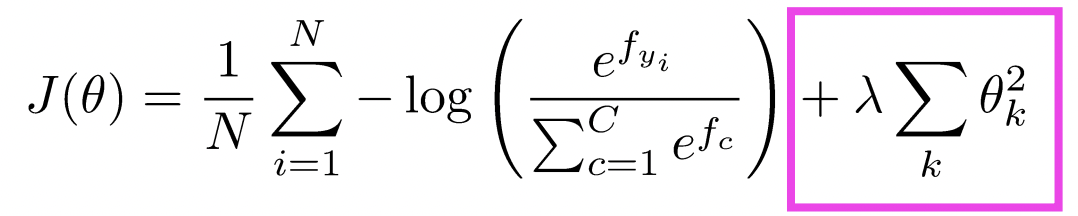
• Uniform reguralization
• L2 penalty는 parameter당 오직 한번 부과된다. 각 example에 대해 각각 부과되는 것이 아니다.

🔗 Dropout

• Feature co-adaptation을 방지하는 좋은 regularization method이다.
• Training time : 각 instance마다 random하게 50%의 neuron을 끈다.
• Test time : Training data에서 사용한 것의 2배를 사용하기 때문에 model weights를 반으로 줄인다.
• Feature co-adaptation을 막는다. Feature는 특정 다른 feature가 있는 경우에만 useful할 수 없다. 왜냐하면 feature들이 매번 random하게 사라지기 때문에 model은 서로 다른 example에 대해 어떤 feature가 존재할지 guarantee할 수 없다.
• Model bagging/ensemble model의 형태로 생각할 수 있다.
• 요즘 dropout을 매우 강한 feature-dependent regularizer로 사용한다.
  • Feature-dependent regularizer : 서로 다른 featuresms performance를 maximize하기 위해 다른 정도로 regularized될 수 있다.
  • 그리고 얼마나 많이 regularized될지는 그 feature가 얼마나 사용되는지에 따라 달려있다. 적게 사용되는 feature들은 많이 regularize하게 된다.

🔗 Vectorization

• Neural network가 빠르게 동작하길 원하면 vector, matrices, tensors를 사용하고 for loop를 사용하면 안된다.

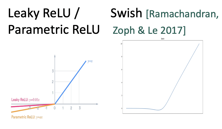
🔗 Non-linearities, old and new

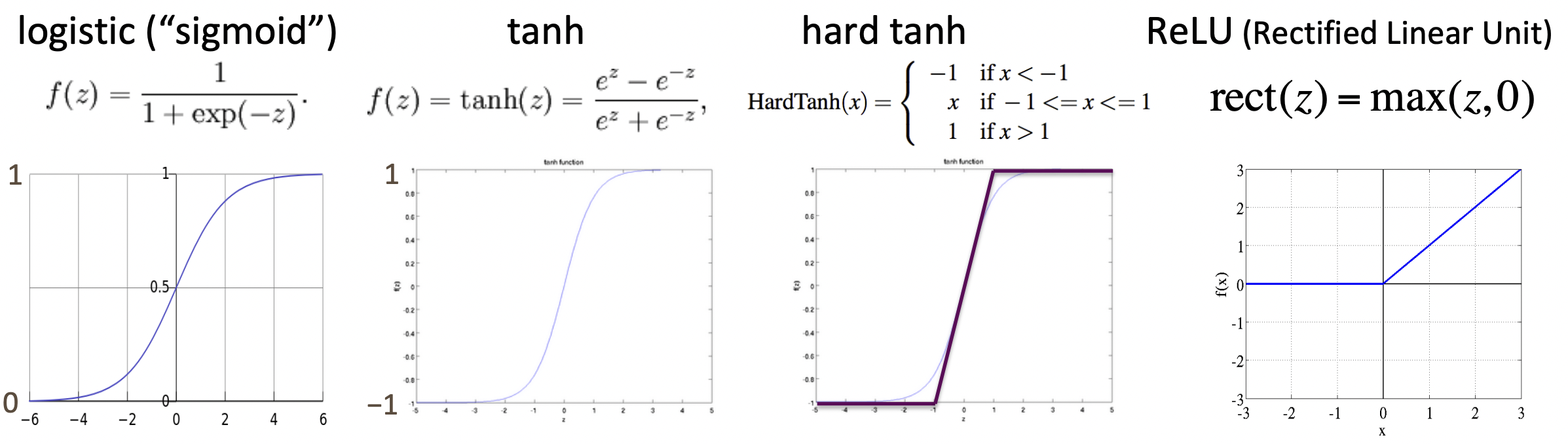
• logistic(sigmoid)의 단점은 다 양수가 된다는 것이다. 그래서 나온 것이 tanh이고 tanh는 logistic을 rescaled하고 shifted하면 얻을 수 있다.
• logistic과 tanh는 exponential을 계산해야하기 때문에 느리고 expensive하다.
• Swish는 거의 ReLU와 같은데 curve가 있다.
• Deep network를 설계할 때 ReLU 먼저 해보자! ReLU가 빠르고 수행도 잘한다.

🔗 Parameter Initialization

• Xavier initialization : 가장 흔한 initialization

🔗 Optimizers

• Differential per-parameter learning rates를 주는 sophisticated adaptive optimizer들이 있다.
  • Adam이 좋다.

🔗 Learning Rates

• Train하면서 Learning rate가 줄어들도록 하는 것이 좋은 결과를 가져올 수 있다.
• Fancier optimizers(like Adam)도 여전히 learning rate를 쓰지만 initial rate일 뿐 optimizer가 점점 shrink하기 때문에 높은 learning rate로 시작하는 것이 좋다.

Language Modeling

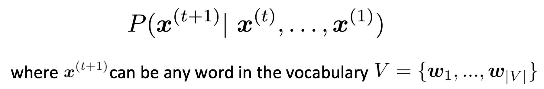
• Language Modeling은 어떤 word가 다음에 나올지를 예측하는 task이다.

• A sequence of words(a preceding context)가 주어졌을 때 다음 word의 probability distribution을 계산한다.
  

• Language modeling을 하는 system을 Language Model이라고 한다.

• Language Model을 a piece of text에 probability를 assign하는 system으로 생각할 수도 있다.

• Text가 있을때 probability of text는 다음과 같다.
  

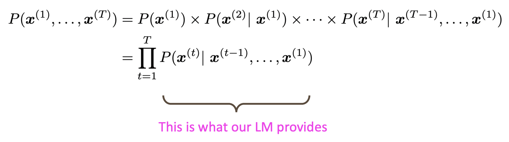
  • Language model이 제공한 각 next word를 predicting한 probability를 곱하여 구할 수 있다.

어떻게 Language Model을 학습할까?
Traditional answer은 n-gram Language Model이다.

n-gram Language Models

🔗 Idea

• 서로 다른 n-gram들이 얼마나 자주 발생했는지 통계를 수집하여 이를 next word를 predict하는데 사용한다.

🔗 과정
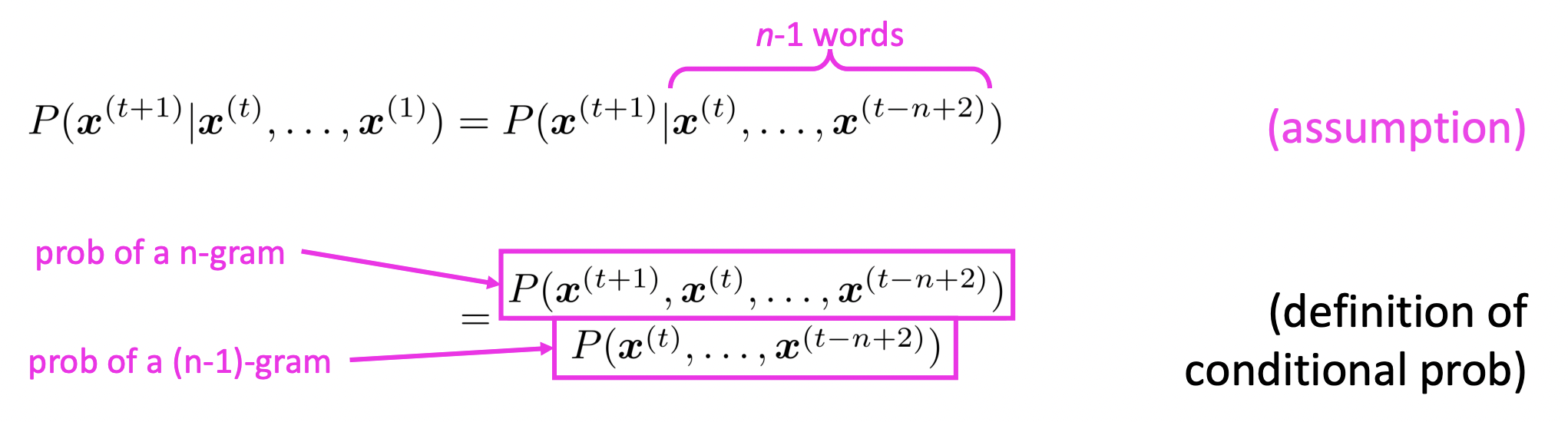
① Markov assumption(markov models)을 한다 : x^(t+1)은 오직 앞에 나온 n-1개의 word에 달려있다.

• 단점 : Predict하는데 도움이 될 수 있는 앞 context가 제거된다.
• n-gram에서 n은 분자의 size이다. Markov model은 context size를 order로 한다.
• 참고 : Naive Bayes model = class specific unigram language model

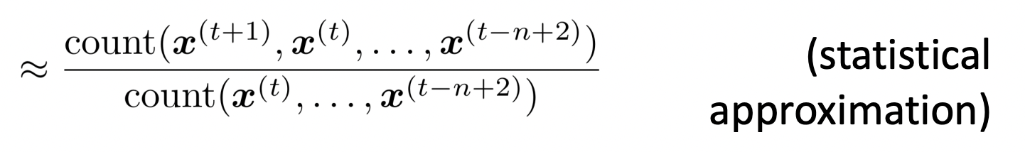
❓ n-gram과 (n-1)-gram probabilities는 어떻게 얻을까?

• large corpus of text에서 센다.
  

🔗 문제 : Sparsity Problems with n-gram Language Models

1. 4-gram language model을 예로 들면, 정말 천문학적인 양을 보지 않은 한 4 word sequences는 본 적 없는 경우가 많을 것이다. 그럼 해당 word는 probability가 0이 될 것이다.

   • (Partial) Solution : small δ를 count에 추가하여 모두를 non-zero로 만든다. 이를 smoothing이라고 부른다.

2. 분모가 0이 되면 어느 word에 대해서도 probability를 계산할 수 없게 된다.

   • (Partial) Solution : "opened their"만 conditioning해보고, 이것도 없으면 "their"만 conditioning해보고 이것도 없으면 모든 conditioning을 잊고 unigram model을 사용한다. 이를 backoff라고 한다.

즉, 우리가 보지 못한 context에 대해서는 어떠한 probability도 유용하게 계산할 수 없다.
n을 증가하면, sparsity problem을 더 악화시킨다. 보통 초기에는 trigram model을 사용하였고 많은 양의 text data를 수집할 수 있자, 5-gram model을 주로 사용하였다.

🔗 문제 : Storage Problems with n-gram Language Models
corpus에서 본 모든 n-grams에 대한 count를 저장해야한다.n을 늘리거나 corpus를 늘리면 model size가 증가한다.

🔗 Generating text with a n-gram Language Model

• 나온 probability distribution에서 next word를 sampling한다.
  

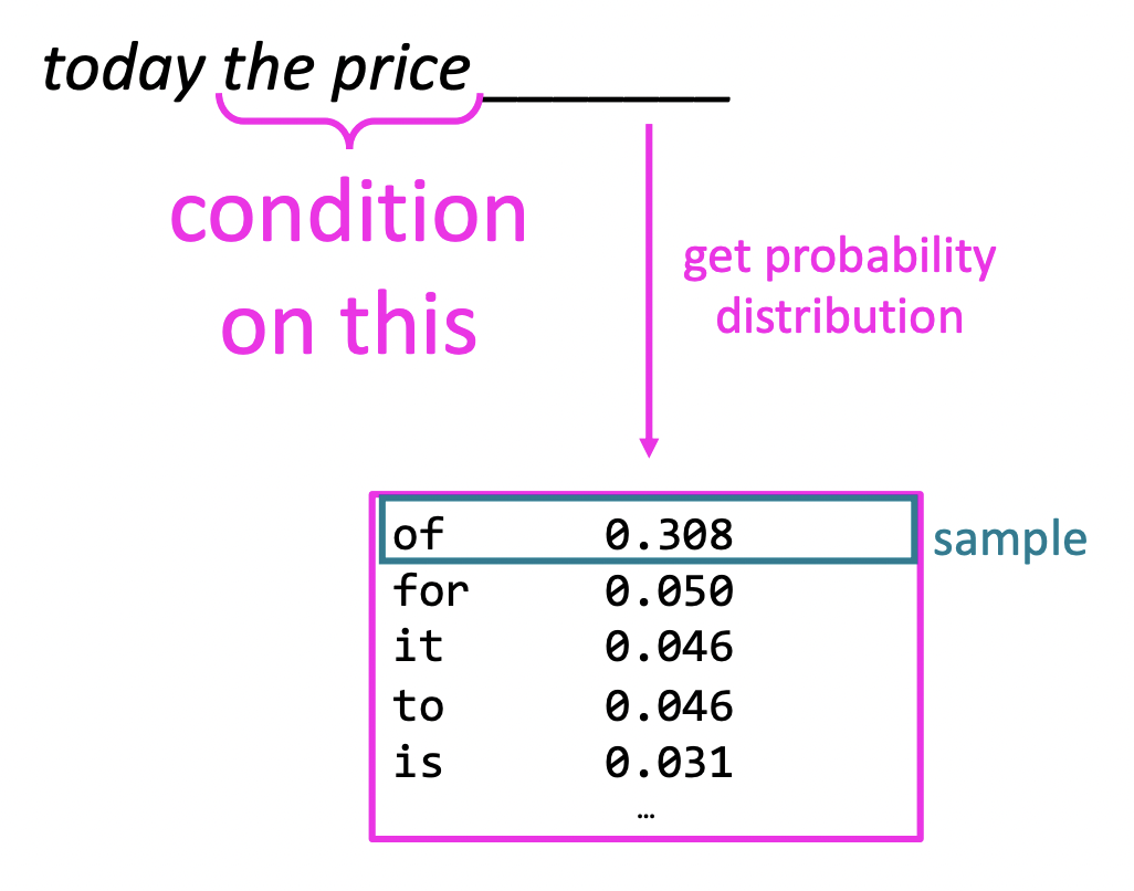
  • Simple trigram Language Model이라고 가정한다.

• Simple n-gram에서 한 것 치고는 꽤 괜찮은 grammatical text가 생성된다.

• 하지만 논리가 일관되지 않고 말이 안된다.

➡️ 더 좋은 language model이 필요하다.

그럼 neural Language Model을 구축하면 어떨까?
가장 간단하게 시도해볼 수 있는 것이 window-based neural model이다.

A fixed-window neural Language Model

• n-gram model처럼 fixed window의 바깥쪽은 버린다.
• neural nets for NLP 초기에 유명했던 모델이다.

🔗 과정

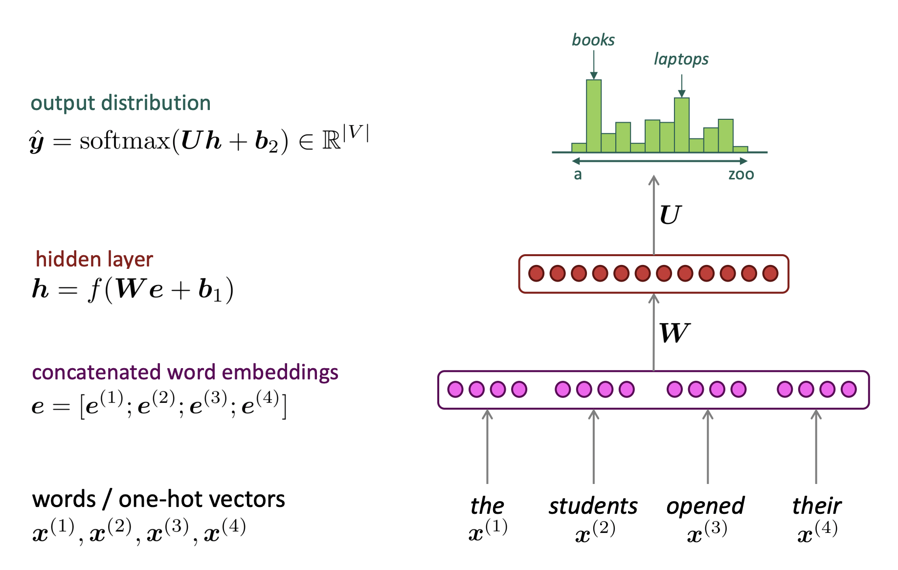
① fixed window를 neural network에 넣는다.
② word embeddings를 concatenate하여 hidden layer에 넣는다.
③ 전체 vocabulary에 대하여 softmax classifier를 하여 probability distribution을 얻는다.

🔗 Improvement over n-gram Language Model

• No sparsity problem
• 모든 관찰된 n-grams를 저장할 필요가 없다. 단순히 word vectors와 W, U matrices만 저장하면 된다.
• Distributed representations of words의 이점을 챙긴다.
  • Train에서 본 적이 없는 word라고 하더라도 semantically similar words에 대해서 비슷한 probability distribution을 주도록 predict한다.

🔗 Remaining problems

• Fixed window는 너무 작다.
• Window를 확대하면 W가 확대된다.
• Window는 절때 충분히 커질 수 없다.
• x^(1)과 x^(2)는 각자 W에서 완전히 다른 weight들과 곱해진다.
  • context의 각 위치마다 완벽하게 다른 weight를 학습한다.
  • 그래서 모델에는 다른 position에 있는 word들을 어떻게 다루는지에 대한 공유가 없다. 비록 어떤 의미에서 그것들이 적어도 어느 정도 position independent한 semantic 요소들에 기여할지라도 그렇다.
  • word2vec이나 Naive는 word order를 고려하지 않는데, language modeling에서는 word order가 매우 중요하기 때문에 language model에서는 잘 동작하지 않는다.
• input이 처리되는 방식에 symmetry가 없다.

즉, 우리는 word order를 어느정도 사용하기를 원한다. 하지만 이 model은 각 position이 완전히 독립적으로 modeling되는 반대의 극단에 있다.
따라서 임의의 양의 context를 처리하고, 여전히 근접성에 민감한 상태에서 parameter를 더 많이 공유할 수 있는 neural architecture를 원한다.
그것이 바로 Recurrent Neural Network이다.

Recurrent Neural Network

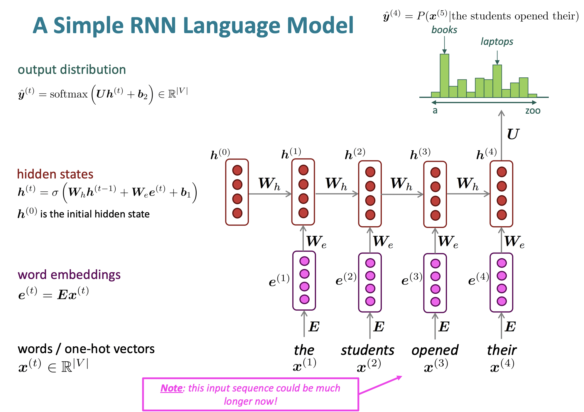
💡 Core idea
same weights W를 반복적으로 적용한다.

• Recurrent의 의미 : hidden layer를 유지하고 feeding the hidden layer back into itself
• 첫번째 word를 기반으로 hidden representation을 계산한다. Second word에 대한 hidden layer를 예측할때는 second word뿐만 아니라 이전 word에 대한 hidden layer도 함께 feed in 한다.
• 이제는 context에 몇 개의 word가 있어도 상관없다.

🔗 과정
① word identity에 대한 one hot vectors를 가지고 있다.
② 각 word에 대해 word embedding을 lookup하여 word embedding을 얻는다.
③ Hidden states에 feed in 한다.

• 가장 많이 쓰이는 non-linearity function은 tanh function이다.
• 첫 번째 word에 대한 hidden layer에 matrix W를 multiply하여 두 번째 word와 같이 들어가서 next hidden state를 generate한다.

④ 어느 position에서든지 hidden vector를 가져와서 softmax layer에 넣어 softmax distribution을 얻는다. 이것이 next word에 대한 probability distribution이다.

🔗 RNN Advantages

• Can process any length input
• Step t에서의 계산에 여러 step 전에 대한 information이 사용될 수 있다.
• 긴 input context에 대해서도 model size는 증가하지 않는다.
  • RNN에는 2개의 parameter가 있다.
    1. input embedding과 multiply하는 matrix
    2. network의 hidden state를 update하기 위한 matrix
• 몇 weight들은 매 timestep에 적용되기 때문에 prediction을 생성하는데 있어서 서로 다른 inputs가 어떻게 처리되는지에 관한 symmetry가 있다.

🔗 RNN Disadvantages

• Recurrent computation이 느리다.
• 실제로는, 여러 step 전에 대한 information에 접근하는 것이 어렵다.

Reference

• CS224n: Natural Language Processing with Deep Learning Lecture at Stanford University