2023.04.24 TIL

토깽이연구소 수석연구원·2023년 4월 24일

React TIL 알고리즘 자료구조

TIL

목록 보기

16/37

오늘의 나는 무엇을 잘했을까?

자료구조와 알고리즘을 천천히, 차근차근 진도를 나가서 오늘 완강하였다. 하지만 계속 복습을 하고 내 것으로 만들 예정이다.

오늘의 나는 무엇을 배웠을까?

이진 탐색 트리

Binary Search Tree라고도 부르며, 모든 노드의 왼쪽 자식 노드에는 노드의 데이터보다 작은 값이, 오른쪽 자식 노드에는 노드의 데이터보다 큰 값이 들어가는 등 규칙이 있어 데이터를 Tree의 높이만큼의 비교 연산을 하면 원하는 데이터를 찾을 수 있어 탐색 트리라고 한다.

이진탐색 트리 구현
- 완전 이진 트리라는 보장이 없기 때문에 배열로 구현하지 않는다.
- 노드 클래스로 구현할 수 있다. 다만 이전에 노드 클래스로 구현했던 트리와 다르게 노드의 부모 노드에 대한 레퍼런스도 저장한다.
이진 탐색 트리 순회
- inorder 순회를 하면 데이터를 정렬된 순서대로 순회할 수 있다.

삽입

어떤 노드를 이진 탐색 트리에 삽입하려면 루트부터 시작하여 이진 탐색 트리의 속성을 유지하면서 자신의 위치를 찾아가면 된다.

새로운 노드 생성
root노드부터 비교하면서 저장할 위치 찾음
찾은 위치에 새롭게 만든 노드 연결

시간 복잡도
- 트리의 높이: h
- 최악의 경우 비교 연산 h+1번
- $O(h)$

코드

def insert(self, data):
  new_node = Node(data)  # 삽입할 데이터를 갖는 새 노드 생성

  # 트리가 비었으면 새로운 노드를 root 노드로 만든다
  if self.root is None:
    self.root = new_node
    return

  # 여기에 코드를 작성하세요
  node_to_compare = self.root
  while True:
    if new_node.data < node_to_compare.data:
      if node_to_compare.left_child is None:
          new_node.parent = node_to_compare
          node_to_compare.left_child = new_node
          break
      node_to_compare = node_to_compare.left_child
    else:
      if node_to_compare.right_child is None:
          new_node.parent = node_to_compare
          node_to_compare.right_child = new_node
          break
      node_to_compare = node_to_compare.right_child

탐색

특정 데이터를 가지는 노드를 찾아 리턴하는 연산

루트노드부터 시작하여 비교를 진행
탐색값 < 노드값 이면 비교 대상 노드를 왼쪽 자식으로 변경
탐색값 == 노드값이면 리턴
탐색값 > 노드값 이면 비교 대상 노드를 오른쪽 자식으로 변경

시간 복잡도: $O(h)$
코드

def search(self, data):
  """이진 탐색 트리 탐색 메소드, 찾는 데이터를 갖는 노드가 없으면 None을 리턴한다"""
  # 여기에 코드를 작성하세요
  node_to_compare = self.root
  while node_to_compare is not None:
    if node_to_compare.data == data:
      return node_to_compare
    elif node_to_compare.data > data:
      node_to_compare = node_to_compare.left_child
    else:
      node_to_compare = node_to_compare.right_child
  return None

삭제

삭제할 노드를 탐색하여 찾은 후 트리에서 지우는 연산
경우1: 삭제하려는 노드가 leaf노드일 때
1. 삭제 대상 노드의 부모 노드의 자식 노드 레퍼런스에 None을 넣는다
경우2: 삭제하려는 데이터 노드가 하나의 자식 노드만 있을 때
1. 삭제 대상 노드의 부모와 자식을 연결시킨다
경우3: 삭제하려는 데이터의 노드가 2개의 자식이 있을 때
1. 석세서 노드를 찾는다(삭제하려는 노드보다 큰 데이터 중 가장 작은 데이터를 가지는 노드)
2. 삭제 대상 노드의 데이터를 석세서 노드의 데이터로 덮어쓴다
3. 석세서 노드를 삭제한다.
시간 복잡도: $O(h)$

코드

def delete(self, data):
    """이진 탐색 트리 삭제 메소드"""
    node_to_delete = self.search(data)  # 삭제할 노드를 가지고 온다
    parent_node = node_to_delete.parent  # 삭제할 노드의 부모 노드

    # 경우 1: 지우려는 노드가 leaf 노드일 때
    if node_to_delete.left_child is None and node_to_delete.right_child is None:
		    if self.root is node_to_delete:
		      self.root = None
    else:  # 일반적인 경우
	      if node_to_delete is parent_node.left_child: 
          parent_node.left_child = None
        else:
          parent_node.right_child = None

    # 경우 2: 지우려는 노드가 자식이 하나인 노드일 때:
    elif node_to_delete.left_child is None:  # 지우려는 노드가 오른쪽 자식만 있을 때:
        # 지우려는 노드가 root 노드일 때
        if node_to_delete is self.root:
            self.root = node_to_delete.right_child
            self.root.parent = None
        # 지우려는 노드가 부모의 왼쪽 자식일 때
        elif node_to_delete is parent_node.left_child:
            parent_node.left_child = node_to_delete.right_child
            node_to_delete.right_child.parent = parent_node
        # 지우려는 노드가 부모의 오른쪽 자식일 때
        else:
            parent_node.right_child = node_to_delete.right_child
            node_to_delete.right_child.parent = parent_node

    elif node_to_delete.right_child is None:  # 지우려는 노드가 왼쪽 자식만 있을 때:
        # 지우려는 노드가 root 노드일 때
        if node_to_delete is self.root:
            self.root = node_to_delete.left_child
            self.root.parent = None
        # 지우려는 노드가 부모의 왼쪽 자식일 때
        elif node_to_delete is parent_node.left_child:
            parent_node.left_child = node_to_delete.left_child
            node_to_delete.left_child.parent = parent_node
        # 지우려는 노드가 부모의 오른쪽 자식일 때
        else:
            parent_node.right_child = node_to_delete.left_child
            node_to_delete.left_child.parent = parent_node

    # 경우 3: 지우려는 노드가 2개의 자식이 있을 때
    else:
        successor = self.find_min(node_to_delete.right_child)  # 삭제하려는 노드의 successor 노드 받아오기

        node_to_delete.data = successor.data  # 삭제하려는 노드의 데이터에 successor의 데이터 저장

        # successor 노드 트리에서 삭제
        if successor is successor.parent.left_child:  # successor 노드가 오른쪽 자식일 때
            successor.parent.left_child = successor.right_child
        else:  # successor 노드가 왼쪽 자식일 때
            successor.parent.right_child = successor.right_child        
    
        if successor.right_child is not None:  # successor 노드가 오른쪽 자식이 있을 떄
            successor.right_child.parent = successor.parent

그래프

그래프는 데이터간 연결 관계를 나타낼 때 사용하는 자료구조이다. 네트워크 통신, 위치 데이터, sns 친구관계 데이터 등을 처리할 때 많이 사용한다. 그래프를 구성하는 두 가지 요소는 노드와 엣지라고 부른다.

노드: 하나의 데이터 단위를 나타내는 객체
엣지: 그래프에서 두 노드의 직접적인 연결 관계 데이터
그래프 용어
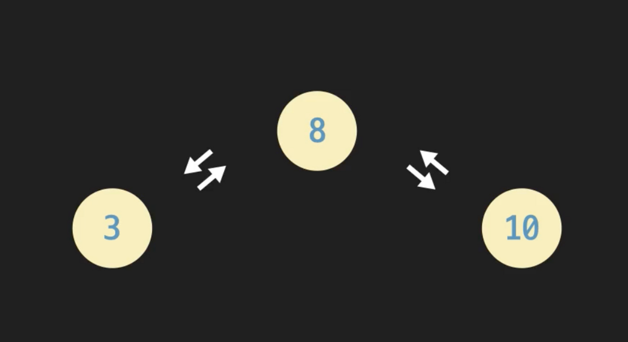
- 인접: 두 노드가 엣지가 있으면, 두 노드는 인접해있다고 한다
- 경로: 두 노드사이의 엣지들로 연결되어있는 루트, 경로의 거리는 엣지의 수로 나타낸다
- 사이클: 특정 노드에서 다른 노드들을 거쳐 다시 특정 노드로 돌아오는 경로
- 차수: 한 노드가 가지고 있는 엣지의 수
방향 그래프(undirected graph)
- 인스타그램의 팔로우 관계와 같이 방향이 있는 그래프
- 경로 또한 방향으로 결정된다.
- 노드의 차수도 입력차수와 출력차수로 나뉜다.
가중치 그래프(weighted graph)
- 엣지에 가중치(weight)가 있다
- 경로의 거리는 경로의 모든 엣지의 가중치들의 합이 된다

그래프 노드 구현

클래스로 구현

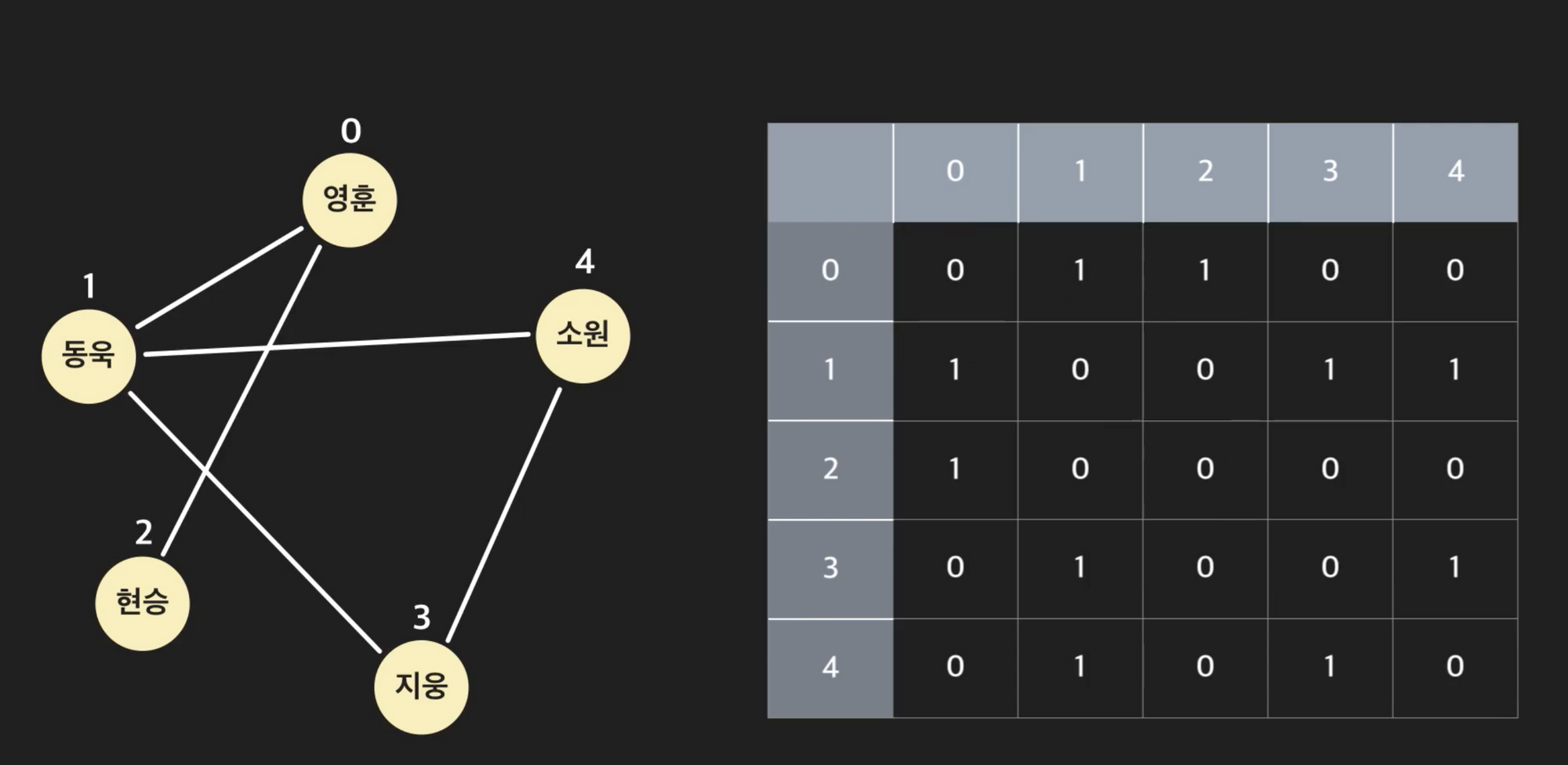
class StationNode:
	def __init__(self, name, num_exits):
		self.name = name
		self.num_exits = num_exits

station_0 = StationNode("교대역", 14)
station_1 = StationNode("사당역", 14)
station_2 = StationNode("종로3가역", 16)
station_3 = StationNode("서울역", 16)

# 노드들을 파이썬 리스트에 저장
stations_list = [station_0, station_1, station_2, station_3]

# 노드들을 해시 테이블에 저장(딕셔너리)
stations_dict = {
    "교대역": station_0,
    "사당역": station_1,
    "종로3가역": station_2,
    "서울역": station_3
}

그래프 엣지 구현: 인접 행렬

인접 행렬은 각 행, 열의 인덱스를 노드의 인덱스로 생각하고, 행렬의 각 셀 데이터에 두 노드의 인접 여부를 1 또는 0으로 저장하는 2차원 배열이다.

예를 들어 3번 노드와 4번노드가 인접해 있다면(사이에 엣지가 존재한다면) 인접행렬의 (3, 4)셀 에는 1이 저장된다. 마찬가지로 (4, 3)셀에도 1이 저장된다.

가중치 그래프의 경우 각 셀에 엣지의 가중치가 저장된다.

방향 그래프의 경우, (3, 4)셀과 (4, 3)셀이 다를 수 있다. 3→4 엣지는 (3, 4)셀에 저장되고 4→3엣지는 (4, 3)셀에 저장된다.
그래프 엣지 구현: 인접 리스트

인접 리스트는 각 노드마다 인접한 노드를 배열로 각각 가지게 하는 것이다. 클래스로 구현한 노드에 adjacent_list와 같은 프로퍼티를 추가해줌으로써 구현할 수 있다.

엣지를 인접 리스트로 구현하면 최악의 경우(우리가 보는 노드가 모든 노드들과 연결되어 있다면) $O(V)$ 의 시간복잡도로 인접노드들을 전부 확인할 수 있다. 하지만 이것은 최악의 경우일 뿐 평균은 훨씬 더 적은 연산으로 알아낼 수 있다. 반대로 인접 행렬을 사용하면 인접 노드들을 모두 확인하려면 $O(V^2)$ 만큼 걸린다. 따라서 노드의 인접 노드들을 전부 확인하는 연산이 많다면 인접 리스트가 조금 더 효율적이라고 할 수 있다.

그래프 탐색

그래프 탐색이란 하나의 시작점 노드에서 연결된 노드들을 모두 찾는 것을 말한다. 그래프 순회라고도 한다. 그래프 탐색을 통해 그래프에 대한 여러 의미 있는 정보들을 알아낼 수 있다. 예를 들면 하나의 노드에 얼마나 많은 노드가 연결되어 있는지, 또는 두 노드 사이의 최단 경로 등을 알 수 있다.

다음 두 가지 알고리즘을 통해 그래프 탐색이 이루어진다.

BFS(너비 우선 탐색) -

O(V + E)

시작 노드를 방문 표시 후, 큐에 넣는다

큐에 아무 노드가 없을 때까지:

큐 가장 앞 노드를 꺼낸다
꺼낸 노드에 인접한 모든 노드들을 보면서
- 처음 방문한 노드면, 노드에 방문표시를 한다
- 큐에 넣는다

def bfs(graph, start_node):
    """시작 노드에서 bfs를 실행하는 함수"""
    queue = deque()  # 빈 큐 생성

    # 일단 모든 노드를 방문하지 않은 노드로 표시
    for station_node in graph.values():
        station_node.visited = False
    
    queue.append(start_node)
    while queue:
      station = queue.popleft()
      for near_station in station.adjacent_stations:
        if not near_station.visited:
          near_station.visited = True
          queue.append(near_station)

DFS(깊이 우선 탐색) -

O(V + E)

시작 노드를 방문 표시 후, 스택에 넣음

스택에 아무 노드가 없을 때까지:

스택 가장 위 노드를 꺼낸다
노드를 방문 표시한다.
인접한 노드들을 보면서:
- 처음 방문한 노드이거나 스택에 없는 노드면 방문처리 후 스택에 넣는다

def dfs(graph, start_node):
    """dfs 함수"""
    stack = deque()  # 빈 스택 생성

    # 모든 노드를 처음 보는 노드로 초기화
    for station_node in graph.values():
        station_node.visited = 0
    start_node.visited = 1
    stack.append(start_node)
    while stack:
      station = stack.pop()
      station.visited = 2
      for near_station in station.adjacent_stations:
        if near_station.visited == 0:
          near_station.visited = 1
          stack.append(near_station)

최단 경로 알고리즘

그래프에서 최단 경로란, 두 노드를 이어주는 모든 경로 중 거리가 가장 작은 경로를 말한다.

비 가중치 그래프에서는 BFS알고리즘을 통해 최단경로를 찾을 수 있고, 가중치 그래프에서는 다익스트라 알고리즘을 이용하여 찾을 수 있다.

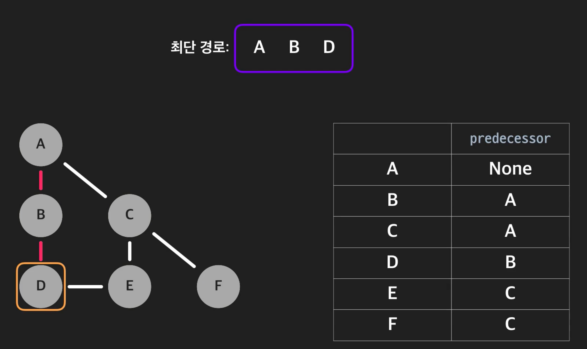
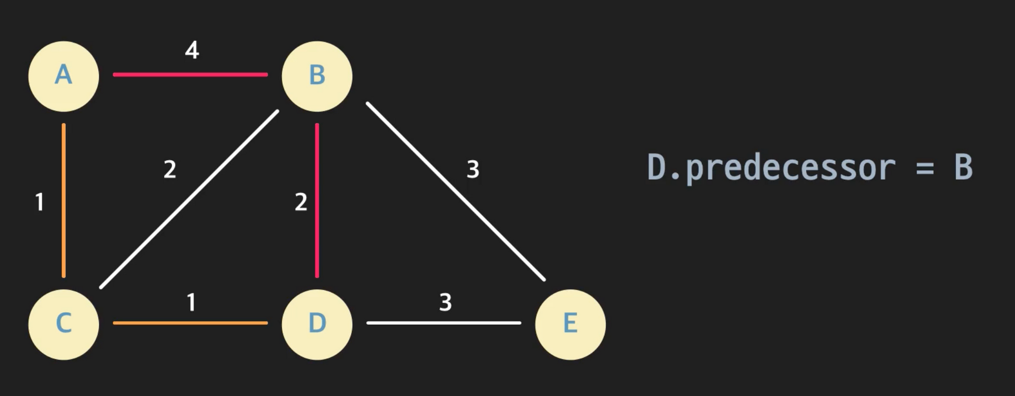
BFS predecessor 변수
- BFS로 최단경로를 찾을 때 필요한 추가 변수
- BFS를 수행하며 특정 노드에 오기 직전의 노드
- 백트래킹 기법을 통해 종착지부터 predecessor를 타고 올라가 시작점을 찾으면 그 경로가 최단 경로이다.

최단 경로용 BFS알고리즘

시작 노드를 방문 표시 후, 큐에 넣음
큐에 아무 노드가 없을 때까지:
- 큐 가장 앞 노드를 꺼낸다
- 꺼낸 노드에 인접한 노드들을 모두 보면서:
  - 처음 방문한 노드면, 방문표시하고, predecessor를 방금 꺼낸 노드로 설정
  - 큐에 넣는다

백트래킹

현재 노드를 경로에 추가한다
현재 노드의 predecessor로 간다
predecessor가 없을 때까지 위 단계를 반복한다

def bfs(graph, start_node):
    """최단 경로용 bfs 함수"""
    queue = deque()  # 빈 큐 생성

    # 모든 노드를 방문하지 않은 노드로 표시, 모든 predecessor는 None으로 초기화
    for station_node in graph.values():
        station_node.visited = False
        station_node.predecessor = None

    # 시작점 노드를 방문 표시한 후 큐에 넣어준다
    start_node.visited = True
    queue.append(start_node)
    
    while queue:  # 큐에 노드가 있을 때까지
        current_station = queue.popleft()  # 큐의 가장 앞 데이터를 갖고 온다
        for neighbor in current_station.adjacent_stations:  # 인접한 노드를 돌면서
            if not neighbor.visited:  # 방문하지 않은 노드면
                neighbor.visited = True  # 방문 표시를 하고
                neighbor.predecessor = current_station
                queue.append(neighbor)  # 큐에 넣는다

def back_track(destination_node):
    """최단 경로를 찾기 위한 back tracking 함수"""
    res_str = destination_node.station_name  # 리턴할 결과 문자열
    current_node = destination_node.predecessor
    while current_node is not None:
        res_str = current_node.station_name + " " + res_str
        current_node = current_node.predecessor
    
    return res_str

stations = create_station_graph("./new_stations.txt")  # stations.txt 파일로 그래프를 만든다

bfs(stations, stations["을지로3가"])  # 지하철 그래프에서 을지로3가역을 시작 노드로 bfs 실행
print(back_track(stations["강동구청"]))  # 을지로3가에서 강동구청역까지 최단 경로 출력

Dijkstra알고리즘
- distance 변수: 특정 노드까지의 최단거리 예상치, 즉 현재까지 찾은 최단 거리 값
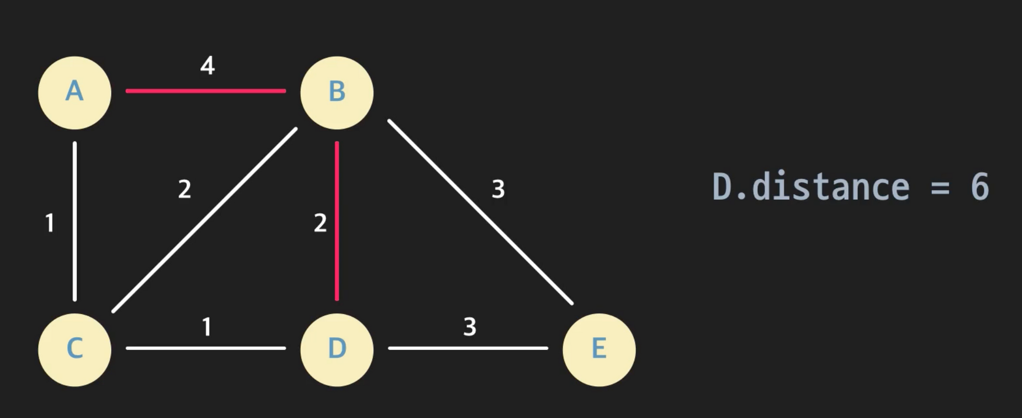
- predecessor 변수: 특정 노드까지 현재까지 찾은 최단 경로상 직전 노드
- complete: 특정 노드까지의 최단 경로를 찾았다고 표시하기 위한 변수
- 엣지 relaxation 예를 들어 a에서 b를 방문하면서 b의 distance, predecessor변수를 갱신해주는 것 위의 예시에서는 엣지 (a, b)를 relax한다 라고 말한다. 엣지 relaxation을 하려면 a.distance + (a, b)의 weight 와 b.distance를 비교해서 전자가 더 작다면 b.distance를 전자로, b.predecessor를 a로 만들어주면 된다.
- 로직
  - 시작점의 distance를 0으로, predecessor를 None으로 초기화
  - 모든 노드가 complete일 때 까지:
    - complete하지 않은 노드 중 distance가 가장 작은 노드 선택
    - 이 노드에 인접한 노드 중 complete하지 않은 노드를 돌면서:
      - 각 엣지를 relax한다
    - 현재 노드를 complete처리한다

Link vs Navigate vs useNavigate

Link 컴포넌트: a 태그로 렌더링 되며, 사용자의 클릭에 반응하는 라우팅을 구현할 때 사용하면 좋습니다. 사용법은 일반 a태그와 같습니다. 그래서 UI와 함께 많이 사용됩니다.

Navigate 컴포넌트: 사용자의 의사와 상관 없이 컴포넌트 렌더링 시 특정 조건을 만족하거나 만족하지 못하면 특정 페이지로 리다이렉션 시킬 때 사용하면 좋습니다. 예를 들면 다음과 같은 코드가 있습니다.

import { Navigate } from 'react-router-dom';

function MyComponent() {
  const isAuthenticated = false;

  return (
    <>
      {isAuthenticated ? (
        <Navigate to="/dashboard" />
      ) : (
        <Navigate to="/login" replace={true} />
      )}
    </>
  );
}