Day 39

Machine Learning Day 14

<Bayesian Inference>

<Bayesian Updating>
When a prior dataset can be roughly represented by a normal distribution, bayesian statistics show that sample information from the same process can be used to obtain a posterior normal distribution. The latter is a weighted combination of the prior and the sample.

<Bayes' Theorem>

=> * Prior Probability: $P(A)$
=> * Likelihood : $P(B|A)$
=> * Posterior Probability: $P(A|B)$
=> * Unnorm Constant: $P(B) \;=\; \sum (joint\;probabilities)$
It can also be

• Joint Probability: $P(A\cap B)$ = Likelihood x Prior Probability
  사전확률을 어떤 행동의 관찰, 정보의 획득에 의해서 사후확률로 업데이트하는것: 베이즈 업데이트

Therefore,

<Exercise.1>

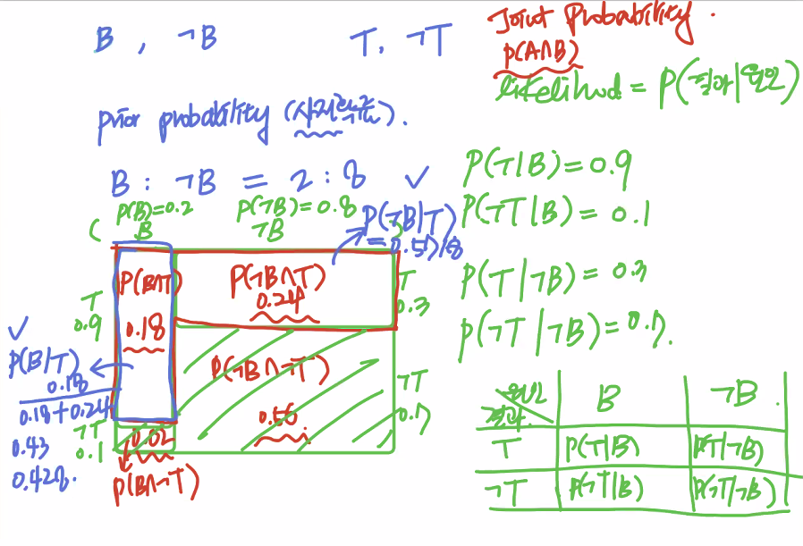
blue: posterial probability (0.428, 0.5718)

-> Probability grew two times bigger with just one more information. 20% -> 43%

<Exercise. 2>

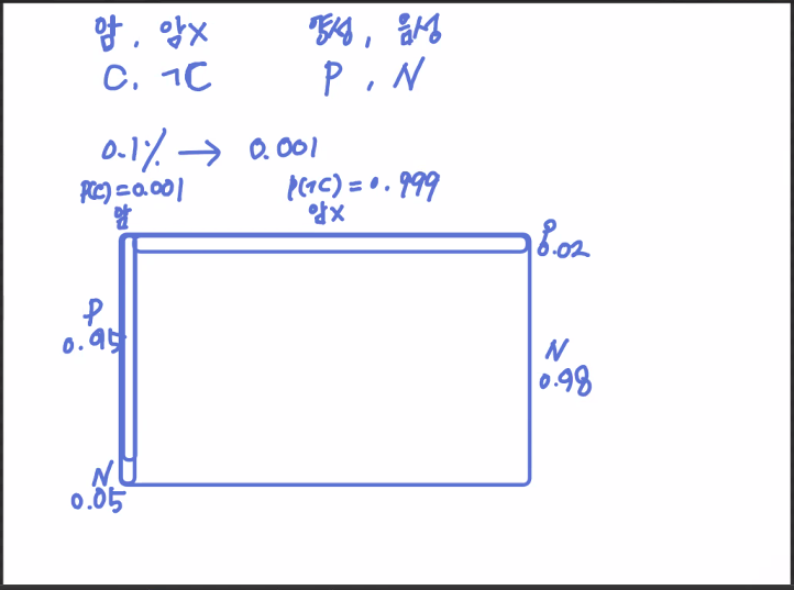
• Prior Probability:

  $P(C)=0.001 \quad P(\neg C)=0.999$

• Likelyhood:

  $P(P|C)=0.95 \quad P(N|C)=0.05 \quad P(P|\neg C)=0.02 \quad P(N|\neg C)=0.98$

• Joint Probability:

  $P(P \cap C) = 0.95 \times 0.001 = 0.00095 \\ P(N \cap C) = 0.05 \times 0.001 = 0.00005 \\ P(P \cap \neg C) = 0.02 \times 0.999 = 0.01998 \\ P(N \cap \neg C) = 0.98 \times 0.999 = 0.97902$

• Posterior Probability:

  $P(C|P) = 0.00095 \; / \; (0.00095+0.01998) = 0.04539 \\P(\neg C|P) = 0.01998 \;/\; (0.00095+0.01998) = 0.0955 \\P(C|N) = 0.00005 \;/\; (0.00005+0.97902) = 0.00005 \\P(\neg C|N) = 0.97902 \;/\; (0.00005+0.97902) = 0.99995$

<Exercise.3>

• Likelihood:

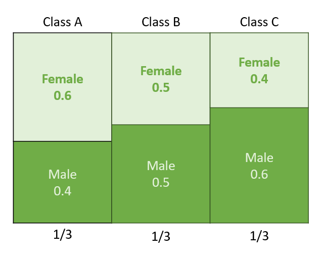
  $P(F|C_{A})=0.6 \quad P(M|C_{A})=0.4 \\P(F|C_{B})=0.5 \quad P(M|C_{B})=0.6 \\P(F|C_{C})=0.4 \quad P(M|C_{C})=0.6$

• Joint Probability:

  $P(F \cap C_{A})= 0.6\times 1/3\;=\;0.2 \quad P(M \cap C_{A})= 0.4\times 1/3\;=\;0.1333 \\P(F \cap C_{B})= 0.5\times 1/3\;=\;0.1666 \quad P(M \cap C_{B})= 0.5\times 1/3\;=\;0.1666 \\P(F \cap C_{C})= 0.4\times 1/3\;=\;0.1333 \quad P(M \cap C_{C})= 0.6\times 1/3\;=\;0.2$

• Posterior Probability:

  $P(C_{A}|F)=0.2 \;/\; (0.2+0.1666+0.1333)=0.40008 \\P(C_{B}|F)=0.1666 \;/\; (0.2+0.1666+0.1333)=0.33326 \\P(C_{C}|F)=0.1333 \;/\; (0.2+0.1666+0.1333)=0.26665$