Logistic Regression with a Neural Network mindset
Backword_propagationForward_propagationLearning_ratePredictionStandardizeinitializeoptimizationsigmoid
Machine_Learning
목록 보기
2/44
Packages
import numpy as np
import copy
import matplotlib.pyplot as plt
import h5py
import scipy
from PIL import Image
from scipy import ndimage
from lr_utils import load_dataset
from public_tests import *

%matplotlib inline
%load_ext autoreload
%autoreload 2
Overview Problem set
아래서 사용하게 될 "data.h5" 데이터셋은
- cat (y=1)과 non-cat (y=0)으로 레이블된 m_train 트레인셋
- cat (y=1)과 non-cat (y=0)으로 레이블된 m_test 테스트셋
- 각각의 이미지는 (num_px, num_px, 3)의 shape을 가진다.
Load data
train_set_x_orig, train_set_y, test_set_x_orig, test_set_y, classes = load_dataset()Example of a picture
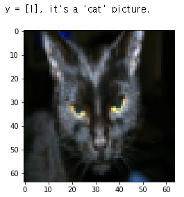
index = 25
plt.imshow(train_set_x_orig[index])
print ("y = " + str(train_set_y[:, index]) + ", it's a '" + classes[np.squeeze(train_set_y[:, index])].decode("utf-8") +  "' picture.")
output:
find the value of <m_train, m_test, num_px>
m_train = train_set_x_orig.shape[0]
m_test = test_set_x_orig.shape[0]
num_px = train_set_x_orig.shape[1]

print ("Number of training examples: m_train = " + str(m_train))
print ("Number of testing examples: m_test = " + str(m_test))
print ("Height/Width of each image: num_px = " + str(num_px))
print ("Each image is of size: (" + str(num_px) + ", " + str(num_px) + ", 3)")
print ("train_set_x shape: " + str(train_set_x_orig.shape))
print ("train_set_y shape: " + str(train_set_y.shape))
print ("test_set_x shape: " + str(test_set_x_orig.shape))
print ("test_set_y shape: " + str(test_set_y.shape))
Number of training examples: m_train = 209
Number of testing examples: m_test = 50
Height/Width of each image: num_px = 64
Each image is of size: (64, 64, 3)
train_set_x shape: (209, 64, 64, 3)
train_set_y shape: (1, 209)
test_set_x shape: (50, 64, 64, 3)
test_set_y shape: (1, 50)
Reshape dataset to flatten image of size(num_px, num_px, 3)->(num_px*num_px**3, 1)
train_set_x_flatten = train_set_x_orig.reshape(train_set_x_orig.shape[0],-1).T
test_set_x_flatten = test_set_x_orig.reshape(test_set_x_orig.shape[0],-1).T
train_set_x_flatten shape: (12288, 209)
train_set_y shape: (1, 209)
test_set_x_flatten shape: (12288, 50)
test_set_y shape: (1, 50)
Standardize dataset
train_set_x = train_set_x_flatten / 255.
test_set_x = test_set_x_flatten / 255.
보편적인 프로세싱 순서:
- 차원과 모양을 알아낸다
- Reshape
- Standardize
General Architecture of the learning algorithm
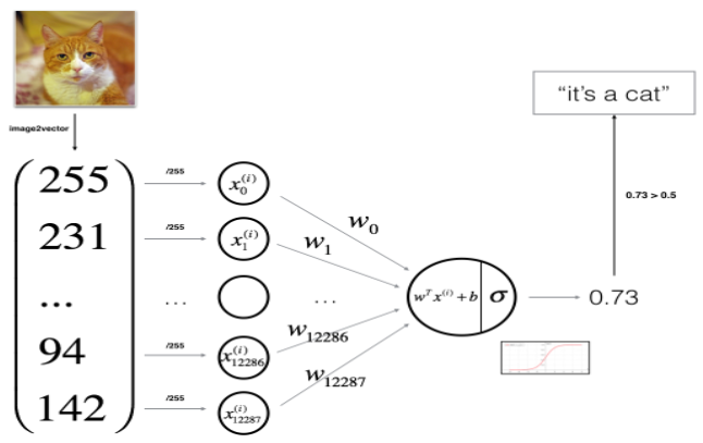
- Initialize parameters
- Learn model by minimizing the cost
- Make predictions (on test set)
- Analyse result
Sigmoid Function
def sigmoid(z):
    s = 1/(1+np.exp(-z))
    return s
Initialize Parameters
def initialize_with_zeros(dim):
w = np.zeros([dim,1])
b = 0.
return w,b
dim = 2
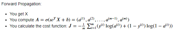
w,b = initialize_with_zeros(dim)Forward and Backward propagation(Compute Cost function)
use:
input:
w - 가중치, array of size(num_px num_px **3, 1)
b - bias
X - 데이터 사이즈 (num_px num_px **3, example 개수)
Y - "label" vector of size(1, example 개수)
.shape[0] 이나 .shape[1]이 헷갈린다면 여기를 참고하자.
def propagate(w, b, X, Y):
#forward propagation
m = X.shape[1]
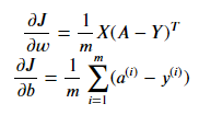
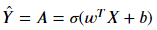
A = sigmoid(np.dot(w.T, X) + b)
cost = -1/m * (np.dot(Y, np.log(A).T) + np.dot((1-Y), np.log(1-A).T))
#backward propagation
dw = 1/m * (np.dot(X, (A-Y).T))
db = 1/m * (np.sum(A-Y))
cost = np.squeeze(np.array(cost))
grads = {"dw":dw, "db":db}
return grads, costOptimization (update parameters)
learn w & b by minimizing the cost function
update rule :
where a is learning rate
def optimize(w, b, X, Y, num_iterations=100, learning_rate=0.009, print_cost=False):
    w = copy.deepcopy(w)
    b = copy.deepcopy(b)

    costs=[]

    for i in range(num_iterations):
        grads, cost = propagate(w, b, X, Y)
        dw = grads["dw"]
        db = grads["db"]

        w = w - learning_rate*dw
        b = b - learning_rate*db

        #Record costs
        if i%100 ==0:
            costs.append(cost)
            if print_cost:
                print(cost)

    params = {"w":w, "b":b}
    grads = {"dw":dw, "db":db}

    return params, grads, costs

params, grads, costs = optimize(w, b, X, Y, num_iterations=100, learning_rate=0.009, print_cost=False)

print ("w = " + str(params["w"]))
print ("b = " + str(params["b"]))
print ("dw = " + str(grads["dw"]))
print ("db = " + str(grads["db"]))
print("Costs = " + str(costs))
Predict
calculate:
convert the entries(data) into 0 or 1
def predict(w, b, X):
    m = X.shape[1] #한 샘플의 차원
    Y_prediction = np.zeros((1, m))
    w = w.reshape(X.shape[0], 1)

    A = sigmoid(np.dot(x.T, X)+b)

    for i in range(A.shape[1]):
        if (A[0,i]>0.5):
            Y_prediction[0,i] = 1
        else:
            Y_prediction[0,i] = 0
    return Y_prediction
Merge All Functions into a model
def model(X_train, Y_train, X_test, Y_test, num_iterations=2000, learning_rate=0.5, print_cost=false):
    w,b = initialize_with_zeros(X_train.shape[0])

    parameters, grads, costs = optimize(w, b, X_train, num_iterations, learning_rate, print_cost)

    w = parameters["w"]
    b = parameters["b"]

    Y_prediction_test = predict(w,b,X_test)
    Y_prediction_train = predict(w,b,X_train)
Analysis
# Plot learning curve (with costs)
costs = np.squeeze(logistic_regression_model['costs'])
plt.plot(costs)
plt.ylabel('cost')
plt.xlabel('iterations (per hundreds)')
plt.title("Learning rate =" + str(logistic_regression_model["learning_rate"]))
plt.show()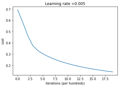
- cost 는 줄어들고 있음(parameters are being learned)
- iterations을 높이면 training set에 대한 정확도는 높아질 수 있지만 test set에 대한 정확도는 낮아진다. => overfitting
Learning Rate
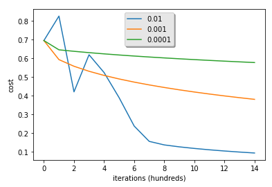
- lr이 너무 크면 그래프가 왔다갔다 할 수 있음.
- lower cost가 더 좋은 모델이 아닐수도 있음. overfitting 인지 아닌지 확인해야 함. (overfitting은 train acc가 test보다 훨씬 클때 가능성이 있음)

뜬금없지만 세계여행이 꿈입니다.