C2W2A1 Optimization Methods
Packages
import numpy as np
import matplotlib.pyplot as plt
import scipy.io
import math
import sklearn
import sklearn.datasets

from opt_utils_v1a import load_params_and_grads, initialize_parameters, forward_propagation, backward_propagation
from opt_utils_v1a import compute_cost, predict, predict_dec, plot_decision_boundary, load_dataset
from copy import deepcopy
from testCases import *
from public_tests import *

%matplotlib inline
plt.rcParams['figure.figsize'] = (7.0, 4.0) # set default size of plots
plt.rcParams['image.interpolation'] = 'nearest'
plt.rcParams['image.cmap'] = 'gray'

%load_ext autoreload
%autoreload 2
Gradient Descent
경사하강법의 update rule은 다음과 같다.
for
for 루프에서 반복자 l이 1에서 시작한다는 점에 유의하자
(첫번째 매개변수는 , 이기 때문)
# GRADED FUNCTION: update_parameters_with_gd

def update_parameters_with_gd(parameters, grads, learning_rate):
    """
    Update parameters using one step of gradient descent

    Arguments:
    parameters -- python dictionary containing your parameters to be updated:
                    parameters['W' + str(l)] = Wl
                    parameters['b' + str(l)] = bl
    grads -- python dictionary containing your gradients to update each parameters:
                    grads['dW' + str(l)] = dWl
                    grads['db' + str(l)] = dbl
    learning_rate -- the learning rate, scalar.

    Returns:
    parameters -- python dictionary containing your updated parameters
    """
    L = len(parameters) // 2 # number of layers in the neural networks

    # Update rule for each parameter
    for l in range(1, L + 1):
        parameters["W" + str(l)] = parameters["W" + str(l)] - learning_rate * grads['dW' + str(l)]
        parameters["b" + str(l)] = parameters["b" + str(l)] - learning_rate * grads['db' + str(l)]

return parameters- (Batch) Gradient Descent:
X = data_input
Y = labels
m = X.shape[1]  # Number of training examples
parameters = initialize_parameters(layers_dims)
for i in range(0, num_iterations):
    # Forward propagation
    a, caches = forward_propagation(X, parameters)
    # Compute cost
    cost_total = compute_cost(a, Y)  # Cost for m training examples
    # Backward propagation
    grads = backward_propagation(a, caches, parameters)
    # Update parameters
    parameters = update_parameters(parameters, grads)
    # Compute average cost
    cost_avg = cost_total / m
- Stochastic Gradient Descent:
X = data_input
Y = labels
m = X.shape[1]  # Number of training examples
parameters = initialize_parameters(layers_dims)
for i in range(0, num_iterations):
    cost_total = 0
    for j in range(0, m):
        # Forward propagation
        a, caches = forward_propagation(X[:,j], parameters)
        # Compute cost
        cost_total += compute_cost(a, Y[:,j])  # Cost for one training example
        # Backward propagation
        grads = backward_propagation(a, caches, parameters)
        # Update parameters
        parameters = update_parameters(parameters, grads)
    # Compute average cost
    cost_avg = cost_total / m
SGD(Stochastic Gradient Descent)는 GD와 달리
전체 훈련세트가 아니라 하나의 훈련샘플만 사용하여 기울기를 업데이트한다.
(미니배치 크기가 1인 미니배치 경사하강법이다)
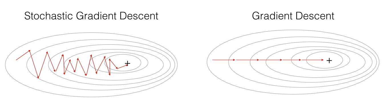
훈련세트가 클 경우, SGD는 계산 속도가 더 빠르다(하나의 훈렴 샘플만 사용하기 때문에)
그러나 매개변수가 부드럽게 수렴하지 않고, 최솟값을 향해 진동한다.
SGD를 구현하려면
1. 반복 횟수
2. 훈련 예제의 수 m
3. 레이어 (부터 까지)
에 대한 3개의 for 루프가 필요하다.
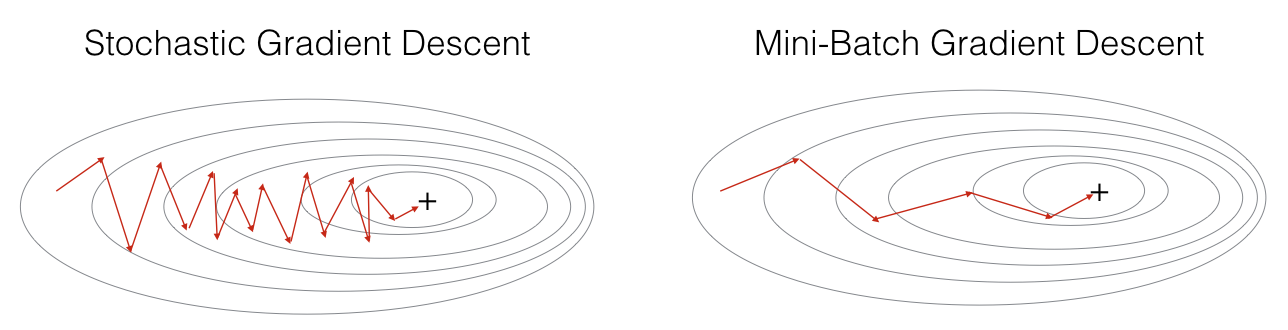
실제로는 1과 m 사이의 적당한 미니배치 크기를 사용한다.
Mini-batch GD를 사용하면, 대부분의 상황에서 SGD보다 더 빨리 최적화할 수 있다
Mini-batch gradient descent
- 미니배치를 생성하는 두 단계
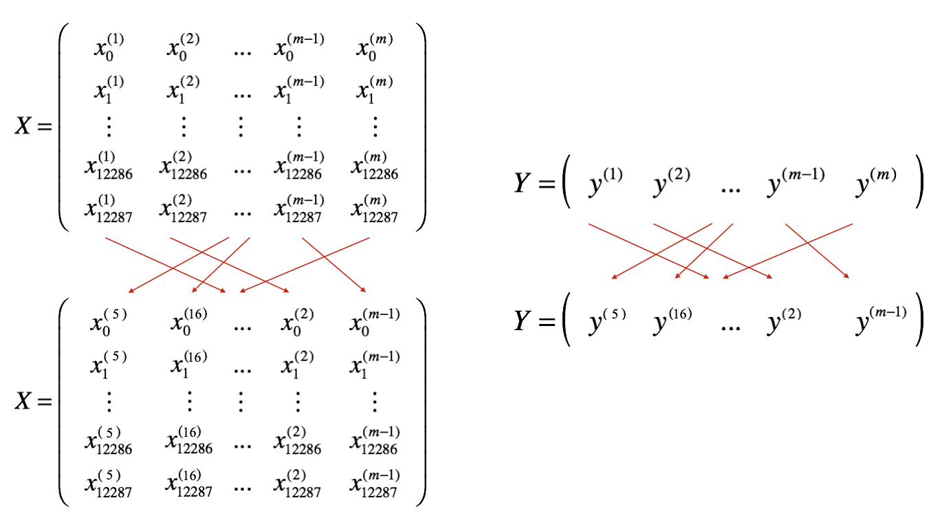
1. Shuffle
훈련 세트 (X, Y)를 무작위로 섞는다. 단, X와 Y를 동기적으로 섞어야 한다.
아래와 같이, X의 i번째 열은 Y에서 i번째 레이블에 해당하는 예제가 되도록 한다.
X와 Y의 인덱스 순서가 같아야 한다.
2. Partition
섞인 (X, Y)를 미니배치 크기(mini_batch_size, 여기서는 64)로 나눈다.
훈련 예제의 수가 mini_batch_size로 나누어 떨어지지 않을 수 있다.
마지막 미니배치 크기가 mini_batch_size보다 작을 경우, 아래와 같은 모습이 된다.
첫 번째 미니배치:  X[:, 0:64], Y[:, 0:64]  # 크기: (input_size, 64), (output_size, 64)
두 번째 미니배치:  X[:, 64:128], Y[:, 64:128]  # 크기: (input_size, 64), (output_size, 64)
...
마지막 미니배치:  X[:, 192:222], Y[:, 192:222]  # 크기: (input_size, 30), (output_size, 30)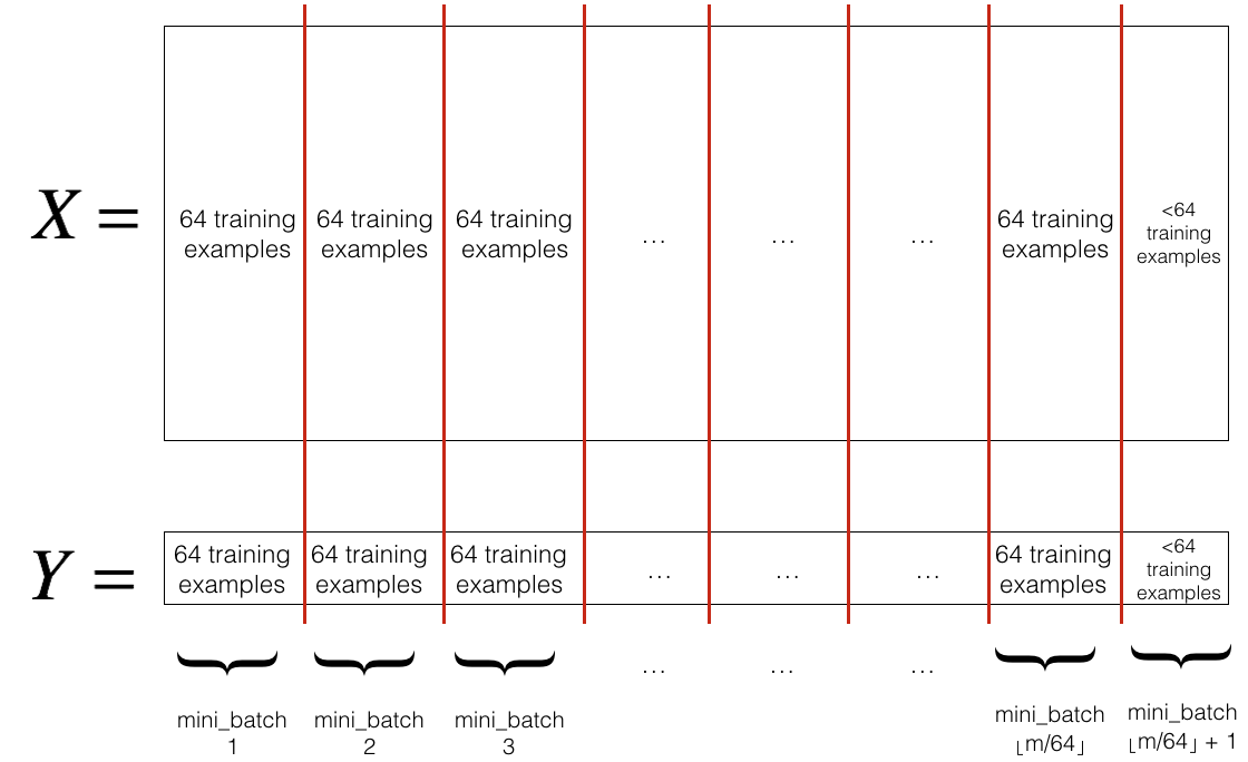
셔플 부분은 이미 구현되어 있다.
1, 2번째 미니배치의 인덱스들을 선택하는 코드는 아래와 같다.
first_mini_batch_X = shuffled_X[:, 0 : mini_batch_size]
second_mini_batch_X = shuffled_X[:, mini_batch_size : 2 * mini_batch_size]
m이 mini_batch_size로 나누어떨어지지 않을 경우
훈련샘플 64개 꽉 찬 미니배치가
개 있으며
마지막 미니배치에 있는 훈련샘플의 개수는
개이다.
위를 참고해서 코드를 짜보자
# GRADED FUNCTION: random_mini_batches

def random_mini_batches(X, Y, mini_batch_size = 64, seed = 0):
    """
    Creates a list of random minibatches from (X, Y)

    Arguments:
    X -- input data, of shape (input size, number of examples)
    Y -- true "label" vector (1 for blue dot / 0 for red dot), of shape (1, number of examples)
    mini_batch_size -- size of the mini-batches, integer

    Returns:
    mini_batches -- list of synchronous (mini_batch_X, mini_batch_Y)
    """

    np.random.seed(seed)            # To make your "random" minibatches the same as ours
    m = X.shape[1]                  # number of training examples
    mini_batches = []

    # Step 1: Shuffle (X, Y)
    permutation = list(np.random.permutation(m))
    shuffled_X = X[:, permutation]
    shuffled_Y = Y[:, permutation].reshape((1, m))

    inc = mini_batch_size

    # Step 2 - Partition (shuffled_X, shuffled_Y).
    # Cases with a complete mini batch size only i.e each of 64 examples.
    num_complete_minibatches = math.floor(m / mini_batch_size) # number of mini batches of size mini_batch_size in your partitionning
    for k in range(0, num_complete_minibatches):
        mini_batch_X = shuffled_X[:, k*mini_batch_size :(k+1)*mini_batch_size]
        mini_batch_Y = shuffled_Y[:, k*mini_batch_size :(k+1)*mini_batch_size]

        mini_batch = (mini_batch_X, mini_batch_Y)
        mini_batches.append(mini_batch)

    # For handling the end case (last mini-batch < mini_batch_size i.e less than 64)
    if m % mini_batch_size != 0:
        mini_batch_X = shuffled_X[:, int(m/mini_batch_size)*mini_batch_size : ]
        mini_batch_Y = shuffled_Y[:, int(m/mini_batch_size)*mini_batch_size : ]

        mini_batch = (mini_batch_X, mini_batch_Y)
        mini_batches.append(mini_batch)
✅ 미니배치를 구성하기 위해 1️⃣ 섞기, 2️⃣ 분할 해야 한다
✅ 미니배치의 크기로는 주로 2의 제곱수를 사용한다 (16, 32, 64, 128)
Momentum
모멘텀 알고리즘은 기존 미니배치 경사하강법의 진동을 줄여준다.
이전 단계 기울기의 지수가중평균은 변수 에 저장된다.
는 산 아래로 굴러내려가는 공의 방향과 속도에 비유할 수 있다.
속도(그리고 모멘텀)이 크면 공은 산에서 가장 낮은 곳에 더 빨리 도착할 수 있을 것이다
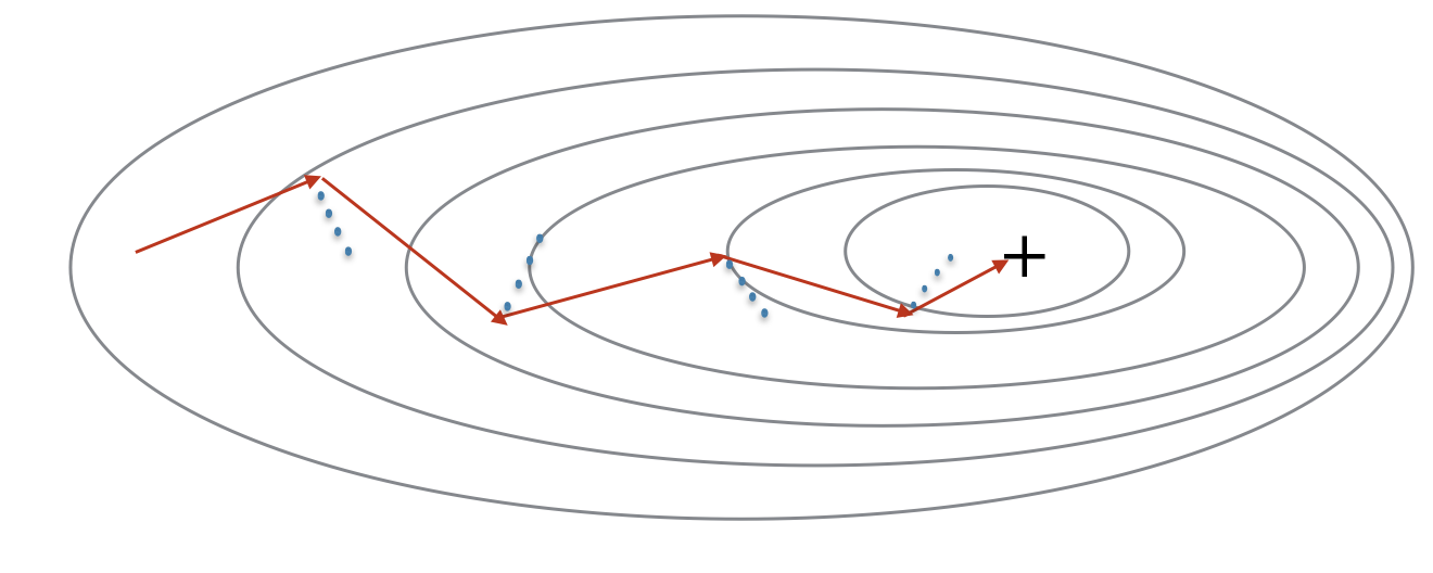
빨간 화살표는 모멘텀을 사용하는 미니배치 경사하강법이 수행하는 한 단계를 보여준다.
파란 점선은 각 단계에서 기울기의 방향을 보여준다.
단순히 기울기를 따라가는 것이 아니라, 기울기는 v에 영향을 미치고, 그 v 방향으로 한 단계를 진행한다.
# GRADED FUNCTION: initialize_velocity

def initialize_velocity(parameters):
    """
    Initializes the velocity as a python dictionary with:
                - keys: "dW1", "db1", ..., "dWL", "dbL"
                - values: numpy arrays of zeros of the same shape as the corresponding gradients/parameters.
    Arguments:
    parameters -- python dictionary containing your parameters.
                    parameters['W' + str(l)] = Wl
                    parameters['b' + str(l)] = bl

    Returns:
    v -- python dictionary containing the current velocity.
                    v['dW' + str(l)] = velocity of dWl
                    v['db' + str(l)] = velocity of dbl
    """

    L = len(parameters) // 2 # number of layers in the neural networks
    v = {}

    # Initialize velocity
    for l in range(1, L + 1):
        v["dW" + str(l)] = np.zeros((parameters["W" + str(l)].shape[0], parameters["W" + str(l)].shape[1]))
        v["db" + str(l)] = np.zeros((parameters["b" + str(l)].shape[0], parameters["b" + str(l)].shape[1]))

    return v
속도 v를 0으로 초기화한다.
- 모멘텀을 사용할 때 매개변수 업데이트 규칙
L은 레이어의 개수, 는 모멘텀, 는 학습률이다.
이번에도 for 루프의 반복자 l은 1부터 시작한다.
# GRADED FUNCTION: update_parameters_with_momentum

def update_parameters_with_momentum(parameters, grads, v, beta, learning_rate):
    """
    Update parameters using Momentum

    Arguments:
    parameters -- python dictionary containing your parameters:
                    parameters['W' + str(l)] = Wl
                    parameters['b' + str(l)] = bl
    grads -- python dictionary containing your gradients for each parameters:
                    grads['dW' + str(l)] = dWl
                    grads['db' + str(l)] = dbl
    v -- python dictionary containing the current velocity:
                    v['dW' + str(l)] = ...
                    v['db' + str(l)] = ...
    beta -- the momentum hyperparameter, scalar
    learning_rate -- the learning rate, scalar

    Returns:
    parameters -- python dictionary containing your updated parameters
    v -- python dictionary containing your updated velocities
    """

    L = len(parameters) // 2 # number of layers in the neural networks

    # Momentum update for each parameter
    for l in range(1, L + 1):
        # compute velocities
        v["dW" + str(l)] = beta*v["dW" + str(l)] + (1-beta)*grads['dW' + str(l)]
        v["db" + str(l)] = beta*v["db" + str(l)] + (1-beta)*grads['db' + str(l)]

        # update parameters
        parameters["W" + str(l)] = parameters["W" + str(l)] - learning_rate*v["dW" + str(l)]
        parameters["b" + str(l)] = parameters["b" + str(l)] - learning_rate*v["db" + str(l)]

    return parameters, v
속도 v는 초기에 0으로 설정된다. 따라서 알고리즘은 몇번의 반복을 거쳐 속도를 누적하고, 점점 더 큰 보폭으로 나아가게 된다.
이면, 모멘텀 없는 일반적인 경사하강법이다.
𝛽 값을 어떻게 선택해야 할까?
-
𝛽가 클수록 업데이트가 더 부드러워지며, 과거의 그라디언트를 더 많이 고려한다.
그러나 𝛽가 너무 크면 업데이트를 너무 많이 완화시킬 수 있다. -
일반적으로 𝛽 값은 0.8부터 0.999 사이로 설정하며, 𝛽=0.9를 기본값으로 사용하면 된다
-
가장 적합한 𝛽 값을 찾으려면, 몇 가지 값을 시도하여 비용 함수 𝐽 값을 줄이는 데 가장 잘 작동하는 𝛽를 알아내야 한다
✅ 모멘텀은 경사 하강법의 단계를 부드럽게 만들기 위해 이전 기울기를 고려한다
✅ 배치 경사 하강법, 미니배치 경사 하강법, 확률적 경사 하강법에 적용할 수 있다
✅ 모멘텀 하이퍼파라미터인 𝛽와 학습률인 𝛼를 잘 조정해야 한다
Adam
Adam은 가장 효과적인 최적화 알고리즘 중 하나로, RMSprop과 모멘텀을 결합한 것이다.
다음과 같이 작동한다:
- 이전 기울기들의 지수가중평균을 계산하고 변수 와 (편향보전 후)에 저장
- 이전 기울기들의 제곱의 지수가중평균을 계산하고 변수 와 (편향보정 전)에 저장
- "1"과 "2"에서 얻은 정보를 결합하여 매개변수를 업데이트
먼저 매개변수를 초기화한다.
# GRADED FUNCTION: initialize_adam

def initialize_adam(parameters) :
    """
    Initializes v and s as two python dictionaries with:
                - keys: "dW1", "db1", ..., "dWL", "dbL"
                - values: numpy arrays of zeros of the same shape as the corresponding gradients/parameters.

    Arguments:
    parameters -- python dictionary containing your parameters.
                    parameters["W" + str(l)] = Wl
                    parameters["b" + str(l)] = bl

    Returns:
    v -- python dictionary that will contain the exponentially weighted average of the gradient. Initialized with zeros.
                    v["dW" + str(l)] = ...
                    v["db" + str(l)] = ...
    s -- python dictionary that will contain the exponentially weighted average of the squared gradient. Initialized with zeros.
                    s["dW" + str(l)] = ...
                    s["db" + str(l)] = ...

    """

    L = len(parameters) // 2 # number of layers in the neural networks
    v = {}
    s = {}

    # Initialize v, s. Input: "parameters". Outputs: "v, s".
    for l in range(1, L + 1):
        v["dW" + str(l)] = np.zeros((parameters["W" + str(l)].shape[0], parameters["W" + str(l)].shape[1]))
        v["db" + str(l)] = np.zeros((parameters["b" + str(l)].shape[0], parameters["b" + str(l)].shape[1]))
        s["dW" + str(l)] = np.zeros((parameters["W" + str(l)].shape[0], parameters["W" + str(l)].shape[1]))
        s["db" + str(l)] = np.zeros((parameters["b" + str(l)].shape[0], parameters["b" + str(l)].shape[1]))

    return v, s
Adam 알고리즘의 업데이트 규칙은 다음과 같다
for :
compute on current mini-batch
모멘텀
편향보정
RMSprop (지수가중평균)
편향보정
매개변수 갱신
# GRADED FUNCTION: update_parameters_with_adam

def update_parameters_with_adam(parameters, grads, v, s, t, learning_rate = 0.01,
                                beta1 = 0.9, beta2 = 0.999,  epsilon = 1e-8):
    """
    Update parameters using Adam

    Arguments:
    parameters -- python dictionary containing your parameters:
                    parameters['W' + str(l)] = Wl
                    parameters['b' + str(l)] = bl
    grads -- python dictionary containing your gradients for each parameters:
                    grads['dW' + str(l)] = dWl
                    grads['db' + str(l)] = dbl
    v -- Adam variable, moving average of the first gradient, python dictionary
    s -- Adam variable, moving average of the squared gradient, python dictionary
    t -- Adam variable, counts the number of taken steps
    learning_rate -- the learning rate, scalar.
    beta1 -- Exponential decay hyperparameter for the first moment estimates
    beta2 -- Exponential decay hyperparameter for the second moment estimates
    epsilon -- hyperparameter preventing division by zero in Adam updates

    Returns:
    parameters -- python dictionary containing your updated parameters
    v -- Adam variable, moving average of the first gradient, python dictionary
    s -- Adam variable, moving average of the squared gradient, python dictionary
    """

    L = len(parameters) // 2                 # number of layers in the neural networks
    v_corrected = {}                         # Initializing first moment estimate, python dictionary
    s_corrected = {}                         # Initializing second moment estimate, python dictionary

    # Perform Adam update on all parameters
    for l in range(1, L + 1):
        # Moving average of the gradients. Inputs: "v, grads, beta1". Output: "v".
        v["dW" + str(l)] = beta1*v["dW" + str(l)] + (1-beta1)*grads['dW' + str(l)]
        v["db" + str(l)] = beta1*v["db" + str(l)] + (1-beta1)*grads['db' + str(l)]

        # Compute bias-corrected first moment estimate. Inputs: "v, beta1, t". Output: "v_corrected".
        v_corrected["dW" + str(l)] = v["dW" + str(l)] / (1-beta1**t)
        v_corrected["db" + str(l)] = v["db" + str(l)] / (1-beta1**t)

        # Moving average of the squared gradients. Inputs: "s, grads, beta2". Output: "s".
        s["dW" + str(l)] = beta2*s["dW" + str(l)] + (1-beta2)*grads['dW' + str(l)]**2
        s["db" + str(l)] = beta2*s["db" + str(l)] + (1-beta2)*grads['db' + str(l)]**2

        # Compute bias-corrected second raw moment estimate. Inputs: "s, beta2, t". Output: "s_corrected".
        s_corrected["dW" + str(l)] = s["dW" + str(l)] / (1-beta2**t)
        s_corrected["db" + str(l)] = s["db" + str(l)] / (1-beta2**t)

        # Update parameters. Inputs: "parameters, learning_rate, v_corrected, s_corrected, epsilon". Output: "parameters".
        parameters["W" + str(l)] = parameters["W" + str(l)] - learning_rate * v_corrected["dW" + str(l)] / (np.sqrt(s_corrected["dW" + str(l)]) + epsilon)
        parameters["b" + str(l)] = parameters["b" + str(l)] - learning_rate * v_corrected["db" + str(l)] / (np.sqrt(s_corrected["db" + str(l)]) + epsilon)


    return parameters, v, s, v_corrected, s_corrected
성능 평가
아래 모델을 사용하여 각 최적화 알고리즘의 성능을 평가해보자
optimizer = "gd" / "momentum" / "adam"으로 설정하여 최적화 기법을 바꿀 수 있다.
def model(X, Y, layers_dims, optimizer, learning_rate = 0.0007, mini_batch_size = 64, beta = 0.9,
beta1 = 0.9, beta2 = 0.999, epsilon = 1e-8, num_epochs = 5000, print_cost = True):
L = len(layers_dims) # number of layers in the neural networks
costs = [] # to keep track of the cost
t = 0 # initializing the counter required for Adam update
seed = 10 # For grading purposes, so that your "random" minibatches are the same as ours
m = X.shape[1] # number of training examples
# Initialize parameters
parameters = initialize_parameters(layers_dims)
# Initialize the optimizer
if optimizer == "gd":
pass # no initialization required for gradient descent
elif optimizer == "momentum":
v = initialize_velocity(parameters)
elif optimizer == "adam":
v, s = initialize_adam(parameters)
# Optimization loop
for i in range(num_epochs):
# Define the random minibatches. We increment the seed to reshuffle differently the dataset after each epoch
seed = seed + 1
minibatches = random_mini_batches(X, Y, mini_batch_size, seed)
cost_total = 0
for minibatch in minibatches:
# Select a minibatch
(minibatch_X, minibatch_Y) = minibatch
# Forward propagation
a3, caches = forward_propagation(minibatch_X, parameters)
# Compute cost and add to the cost total
cost_total += compute_cost(a3, minibatch_Y)
# Backward propagation
grads = backward_propagation(minibatch_X, minibatch_Y, caches)
# Update parameters
if optimizer == "gd":
parameters = update_parameters_with_gd(parameters, grads, learning_rate)
elif optimizer == "momentum":
parameters, v = update_parameters_with_momentum(parameters, grads, v, beta, learning_rate)
elif optimizer == "adam":
t = t + 1 # Adam counter
parameters, v, s, _, _ = update_parameters_with_adam(parameters, grads, v, s,
t, learning_rate, beta1, beta2, epsilon)
cost_avg = cost_total / m
# Print the cost every 1000 epoch
if print_cost and i % 1000 == 0:
print ("Cost after epoch %i: %f" %(i, cost_avg))
if print_cost and i % 100 == 0:
costs.append(cost_avg)
# plot the cost
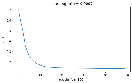
plt.plot(costs)
plt.ylabel('cost')
plt.xlabel('epochs (per 100)')
plt.title("Learning rate = " + str(learning_rate))
plt.show()
return parameterstrain_X, train_Y = load_dataset()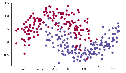
Mini-batch GD
# train 3-layer model
layers_dims = [train_X.shape[0], 5, 2, 1]
parameters = model(train_X, train_Y, layers_dims, optimizer = "gd")

# Predict
predictions = predict(train_X, train_Y, parameters)

# Plot decision boundary
plt.title("Model with Gradient Descent optimization")
axes = plt.gca()
axes.set_xlim([-1.5,2.5])
axes.set_ylim([-1,1.5])
plot_decision_boundary(lambda x: predict_dec(parameters, x.T), train_X, train_Y)
미니배치 경사하강법을 사용하는 모델에서는 update_parameters_with_gd()가 호출된다.
학습 결과는 다음과 같다
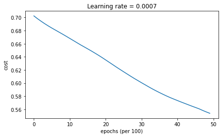

Accuracy: 0.7166666666666667Mini-batch GD with Momentum
모멘텀을 사용하는 미니배치 경사하강법에서는
initialize_velocity(), update_parameters_with_momentum()가 호출된다.
학습 결과는 다음과 같다

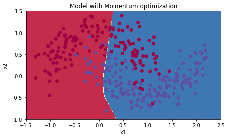
Accuracy: 0.7166666666666667Mini-batch GD with Adam
Accuracy: 0.9433333333333334모멘텀은 대부분의 상황에서 도움이 되지만, 학습률이 작고 훈련세트가 간단할 때에는 일반적인 경사하강법과 크게 다르지 않은 성능을 보인다.
아담은 다른 두 경우에 비해 확연히 좋은 성능을 보인다.
최솟값으로 가장 빠르게 수렴할 뿐 아니라, 메모리를 적게 사용하고 하이퍼파라미터를 조절하기 쉽다는 장점이 있다
Learning Rate Decay
3가지 모델에 학습률 감쇠를 추가해보자
학습률 감쇠는 학습 시 시간이 지남에 따라 학습률 를 점점 감소시켜, 최솟값 주변의 더 좁은 영역에서 진동하도록 하는 방법이다.
이전에 사용한 모델에 decay, decay_rate를 추가하였다
def model(X, Y, layers_dims, optimizer, learning_rate = 0.0007, mini_batch_size = 64, beta = 0.9,
beta1 = 0.9, beta2 = 0.999, epsilon = 1e-8, num_epochs = 5000, print_cost = True, decay=None, decay_rate=1):
"""
3-layer neural network model which can be run in different optimizer modes.
Arguments:
X -- input data, of shape (2, number of examples)
Y -- true "label" vector (1 for blue dot / 0 for red dot), of shape (1, number of examples)
layers_dims -- python list, containing the size of each layer
learning_rate -- the learning rate, scalar.
mini_batch_size -- the size of a mini batch
beta -- Momentum hyperparameter
beta1 -- Exponential decay hyperparameter for the past gradients estimates
beta2 -- Exponential decay hyperparameter for the past squared gradients estimates
epsilon -- hyperparameter preventing division by zero in Adam updates
num_epochs -- number of epochs
print_cost -- True to print the cost every 1000 epochs
Returns:
parameters -- python dictionary containing your updated parameters
"""
L = len(layers_dims) # number of layers in the neural networks
costs = [] # to keep track of the cost
t = 0 # initializing the counter required for Adam update
seed = 10 # For grading purposes, so that your "random" minibatches are the same as ours
m = X.shape[1] # number of training examples
lr_rates = []
learning_rate0 = learning_rate # the original learning rate
# Initialize parameters
parameters = initialize_parameters(layers_dims)
# Initialize the optimizer
if optimizer == "gd":
pass # no initialization required for gradient descent
elif optimizer == "momentum":
v = initialize_velocity(parameters)
elif optimizer == "adam":
v, s = initialize_adam(parameters)
# Optimization loop
for i in range(num_epochs):
# Define the random minibatches. We increment the seed to reshuffle differently the dataset after each epoch
seed = seed + 1
minibatches = random_mini_batches(X, Y, mini_batch_size, seed)
cost_total = 0
for minibatch in minibatches:
# Select a minibatch
(minibatch_X, minibatch_Y) = minibatch
# Forward propagation
a3, caches = forward_propagation(minibatch_X, parameters)
# Compute cost and add to the cost total
cost_total += compute_cost(a3, minibatch_Y)
# Backward propagation
grads = backward_propagation(minibatch_X, minibatch_Y, caches)
# Update parameters
if optimizer == "gd":
parameters = update_parameters_with_gd(parameters, grads, learning_rate)
elif optimizer == "momentum":
parameters, v = update_parameters_with_momentum(parameters, grads, v, beta, learning_rate)
elif optimizer == "adam":
t = t + 1 # Adam counter
parameters, v, s, _, _ = update_parameters_with_adam(parameters, grads, v, s,
t, learning_rate, beta1, beta2, epsilon)
cost_avg = cost_total / m
if decay:
learning_rate = decay(learning_rate0, i, decay_rate)
# Print the cost every 1000 epoch
if print_cost and i % 1000 == 0:
print ("Cost after epoch %i: %f" %(i, cost_avg))
if decay:
print("learning rate after epoch %i: %f"%(i, learning_rate))
if print_cost and i % 100 == 0:
costs.append(cost_avg)
# plot the cost
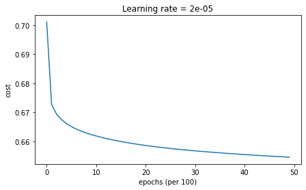
plt.plot(costs)
plt.ylabel('cost')
plt.xlabel('epochs (per 100)')
plt.title("Learning rate = " + str(learning_rate))
plt.show()
return parametersDecay on Every Iteration
학습률은 다음과 같은 식에 따라 업데이트한다. (exponential lerning rate decay)
# GRADED FUNCTION: update_lr

def update_lr(learning_rate0, epoch_num, decay_rate):
    """
    Calculates updated the learning rate using exponential weight decay.

    Arguments:
    learning_rate0 -- Original learning rate. Scalar
    epoch_num -- Epoch number. Integer
    decay_rate -- Decay rate. Scalar

    Returns:
    learning_rate -- Updated learning rate. Scalar
    """

    learning_rate = 1 / (1+decay_rate*epoch_num) * learning_rate0

    return learning_rate
다음 코드블럭을 실행시키면
learning_rate = 0.5
print("Original learning rate: ", learning_rate)
epoch_num = 2
decay_rate = 1
learning_rate_2 = update_lr(learning_rate, epoch_num, decay_rate)

print("Updated learning rate: ", learning_rate_2)

update_lr_test(update_lr)
출력
Original learning rate:  0.5
Updated learning rate:  0.16666666666666666
학습률이 잘 업데이트되는 것을 확인할 수 있다
다음 코드블럭을 실행해 학습률 감쇠를 사용한 미니배치 경사하강법 모델을 학습시킨다
# train 3-layer model
layers_dims = [train_X.shape[0], 5, 2, 1]
parameters = model(train_X, train_Y, layers_dims, optimizer = "gd", learning_rate = 0.1, num_epochs=5000, decay=update_lr)

# Predict
predictions = predict(train_X, train_Y, parameters)

# Plot decision boundary
plt.title("Model with Gradient Descent optimization")
axes = plt.gca()
axes.set_xlim([-1.5,2.5])
axes.set_ylim([-1,1.5])
plot_decision_boundary(lambda x: predict_dec(parameters, x.T), train_X, train_Y)
결과는 다음과 같다.
Accuracy: 0.6533333333333333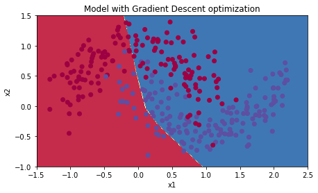
학습률 감쇠가 없을 때보다 더 빠르게 최솟값으로 수렴하는 경향을 보인다
매 반복마다 학습률 를 감쇠시키면, 학습률이 초기에 매우 큰 값(0.1)로 시작했음에도 불구하고 0으로 매우 빠르게 내려간다. 여기서는 문제가 없지만, 에포크의 수가 많을 경우 알고리즘이 업데이트를 멈추는 문제가 발생할 수 있다.
이 문제를 해결하기 위한 방법이 fixed interval scheduling이다.
Fixed Interval scheduling
특정 시간 간격마다 학습률을 감쇠시켜, 학습률이 너무 빠르게 0에 가까워지는 문제를 해결할 수 있다.
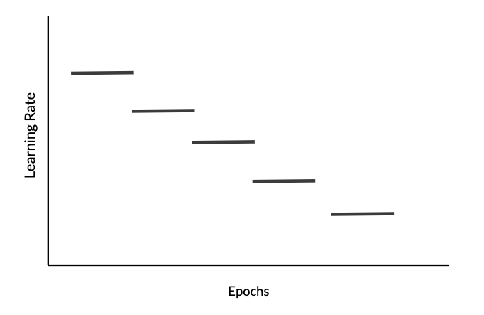
학습률을 다음 식으로 업데이트한다.
epochNum이 timeInterval의 배수일 경우에만 학습률이 감쇠한다.
floor 연산은 numpy.floor()를 사용한다
# GRADED FUNCTION: schedule_lr_decay

def schedule_lr_decay(learning_rate0, epoch_num, decay_rate, time_interval=1000):
    """
    Calculates updated the learning rate using exponential weight decay.

    Arguments:
    learning_rate0 -- Original learning rate. Scalar
    epoch_num -- Epoch number. Integer.
    decay_rate -- Decay rate. Scalar.
    time_interval -- Number of epochs where you update the learning rate.

    Returns:
    learning_rate -- Updated learning rate. Scalar
    """
    learning_rate = 1 / (1 + decay_rate * np.floor(epoch_num/time_interval))* learning_rate0

    return learning_rate
다음 코드블럭을 실행하면
learning_rate = 0.5
print("Original learning rate: ", learning_rate)

epoch_num_1 = 10
epoch_num_2 = 100
decay_rate = 0.3
time_interval = 100
learning_rate_1 = schedule_lr_decay(learning_rate, epoch_num_1, decay_rate, time_interval)
learning_rate_2 = schedule_lr_decay(learning_rate, epoch_num_2, decay_rate, time_interval)
print("Updated learning rate after {} epochs: ".format(epoch_num_1), learning_rate_1)
print("Updated learning rate after {} epochs: ".format(epoch_num_2), learning_rate_2)

schedule_lr_decay_test(schedule_lr_decay)
출력
Original learning rate:  0.5
Updated learning rate after 10 epochs:  0.5
Updated learning rate after 100 epochs:  0.3846153846153846
학습률이 이전보다 느리게 감쇠하는 것을 확인할 수 있다
Mini-batch GD + Learning Rate Decay
다음을 실행시켜 학습률 감쇠를 적용한 미니배치 경사하강법 모델을 학습시킨다
# train 3-layer model
layers_dims = [train_X.shape[0], 5, 2, 1]
parameters = model(train_X, train_Y, layers_dims, optimizer = "gd", learning_rate = 0.1, num_epochs=5000, decay=schedule_lr_decay)

# Predict
predictions = predict(train_X, train_Y, parameters)

# Plot decision boundary
plt.title("Model with Gradient Descent optimization")
axes = plt.gca()
axes.set_xlim([-1.5,2.5])
axes.set_ylim([-1,1.5])
plot_decision_boundary(lambda x: predict_dec(parameters, x.T), train_X, train_Y)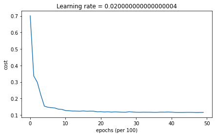
Accuracy: 0.9433333333333334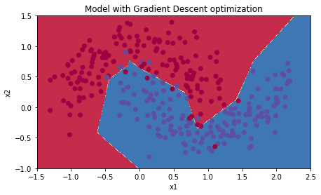
Momentum + Learning Rate Decay
# train 3-layer model
layers_dims = [train_X.shape[0], 5, 2, 1]
parameters = model(train_X, train_Y, layers_dims, optimizer = "momentum", learning_rate = 0.1, num_epochs=5000, decay=schedule_lr_decay)

# Predict
predictions = predict(train_X, train_Y, parameters)

# Plot decision boundary
plt.title("Model with Gradient Descent with momentum optimization")
axes = plt.gca()
axes.set_xlim([-1.5,2.5])
axes.set_ylim([-1,1.5])
plot_decision_boundary(lambda x: predict_dec(parameters, x.T), train_X, train_Y)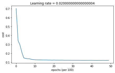
Accuracy: 0.9533333333333334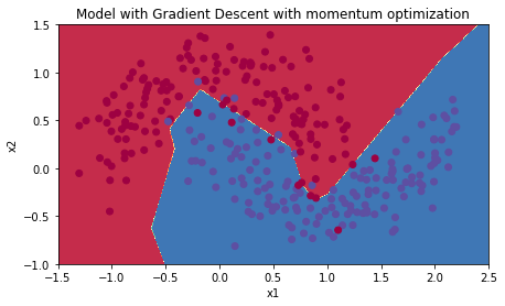
Adam + Learning Rate Decay
# train 3-layer model
layers_dims = [train_X.shape[0], 5, 2, 1]
parameters = model(train_X, train_Y, layers_dims, optimizer = "adam", learning_rate = 0.01, num_epochs=5000, decay=schedule_lr_decay)
# Predict
predictions = predict(train_X, train_Y, parameters)
# Plot decision boundary
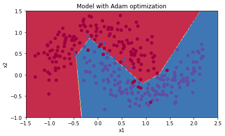
plt.title("Model with Adam optimization")
axes = plt.gca()
axes.set_xlim([-1.5,2.5])
axes.set_ylim([-1,1.5])
plot_decision_boundary(lambda x: predict_dec(parameters, x.T), train_X, train_Y)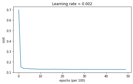
Accuracy: 0.94
학습률 감쇠를 적용한 결과, 미니배치와 모멘텀 모델은 정확성이 크게 증가하였다.
Adam의 경우 정확도는 비슷하지만 더 빠르게 최솟값으로 수렴한다
| optimization method | accuracy |
| Gradient descent | >94.6% |
| Momentum | >95.6% |
| Adam | 94% |
