이 글은 파이썬 머신러닝 완벽 가이드 책 내용을 기반으로 정리했습니다.
내용출처 : 파이썬 머신러닝 완벽가이드
- 디시젼트리를 회귀에 적용한 회귀 트리는 RSS(오차 제곱합)를 가장 잘 줄일 수 있는 변수를 기준으로 분기를 만들어 결과를 예측하는 매우 단순한 모델이다. 어떤 변수가 중요한지, 변수의 값에 따라 예측 결과가 무엇인지 한눈에 볼 수 있어 설명력이 좋은 장점이 있다.
회귀 트리
from sklearn.datasets import load_boston
from sklearn.model_selection import cross_val_score
from sklearn.ensemble import RandomForestRegressor
import pandas as pd
import numpy as np
1. 보스턴 데이터 세트 로드
boston = load_boston()
bostonDF = pd.DataFrame(boston.data, columns = boston.feature_names)

print(bostonDF.shape)
bostonDF.head(3)
(506, 13)| CRIM | ZN | INDUS | CHAS | NOX | RM | AGE | DIS | RAD | TAX | PTRATIO | B | LSTAT | |
|---|---|---|---|---|---|---|---|---|---|---|---|---|---|
| 0 | 0.00632 | 18.0 | 2.31 | 0.0 | 0.538 | 6.575 | 65.2 | 4.0900 | 1.0 | 296.0 | 15.3 | 396.90 | 4.98 |
| 1 | 0.02731 | 0.0 | 7.07 | 0.0 | 0.469 | 6.421 | 78.9 | 4.9671 | 2.0 | 242.0 | 17.8 | 396.90 | 9.14 |
| 2 | 0.02729 | 0.0 | 7.07 | 0.0 | 0.469 | 7.185 | 61.1 | 4.9671 | 2.0 | 242.0 | 17.8 | 392.83 | 4.03 |
# target 데이터프레임 생성
bostonDF['PRICE'] = boston.target
y_target = bostonDF['PRICE']

# feature 데이터프레임에서는 PRICE 컬럼 삭제
X_data = bostonDF.drop(['PRICE'], axis=1,inplace=False)
2. 학습 및 평가 : RandomForestRegressor 회귀트리 모델
# 학습 모델 : RandomForestRegressor
rf = RandomForestRegressor(random_state=0, n_estimators=1000)

# 학습 및 평가 (cross_val_score : MSE를 리스트 형태로 반환해줌 )
neg_mse_scores = cross_val_score(rf, X_data, y_target, scoring="neg_mean_squared_error", cv = 5)
rmse_scores  = np.sqrt(-1 * neg_mse_scores)
avg_rmse = np.mean(rmse_scores)

print(' 5 교차 검증의 개별 Negative MSE scores: ', np.round(neg_mse_scores, 2))
print(' 5 교차 검증의 개별 RMSE scores : ', np.round(rmse_scores, 2))
print(' 5 교차 검증의 평균 RMSE : {0:.3f} '.format(avg_rmse))
5 교차 검증의 개별 Negative MSE scores: [ -7.88 -13.14 -20.57 -46.23 -18.88]
5 교차 검증의 개별 RMSE scores : [2.81 3.63 4.54 6.8 4.34]
5 교차 검증의 평균 RMSE : 4.423 4. 여러 트리회귀 클래스 예측 후 비교
from sklearn.tree import DecisionTreeRegressor
from sklearn.ensemble import RandomForestRegressor
from sklearn.ensemble import GradientBoostingRegressor
from xgboost import XGBRegressor
from lightgbm import LGBMRegressor
# cross_val_score로 교차검증 학습 후 평가지표로 RMSE를 알려주는 함수
def get_model_cv_prediction(model, X_data, y_target):
neg_mse_scores = cross_val_score(model, X_data, y_target, scoring="neg_mean_squared_error", cv = 5)
rmse_scores = np.sqrt(-1 * neg_mse_scores)
avg_rmse = np.mean(rmse_scores)
print('##### ', model.__class__.__name__ , ' #####')
print(' 교차 검증의 평균 RMSE : {0:.3f} '.format(avg_rmse), '\n')dt_reg = DecisionTreeRegressor(random_state=0, max_depth=4)
rf_reg = RandomForestRegressor(random_state=0, n_estimators=1000)
gb_reg = GradientBoostingRegressor(random_state=0, n_estimators=1000)
xgb_reg = XGBRegressor(n_estimators=1000)
lgb_reg = LGBMRegressor(n_estimators=1000)
# 트리 기반의 회귀 모델을 반복하면서 평가 수행
models = [dt_reg, rf_reg, gb_reg, xgb_reg, lgb_reg]
for model in models:
get_model_cv_prediction(model, X_data, y_target)##### DecisionTreeRegressor #####
교차 검증의 평균 RMSE : 5.978
##### RandomForestRegressor #####
교차 검증의 평균 RMSE : 4.423
##### GradientBoostingRegressor #####
교차 검증의 평균 RMSE : 4.269
##### XGBRegressor #####
교차 검증의 평균 RMSE : 4.251
##### LGBMRegressor #####
교차 검증의 평균 RMSE : 4.646
->
디시젼트리보다는 랜덤포레스트 성능이 좋다.
제일 성능이 좋은 모델은 XGBRegressor이다.
5. 트리회귀의 피처 중요도 확인
회귀 트리는 선형 회귀의 회귀 계수 대신, featureimportances로 피처의 중요도를 알 수 있습니다.
import seaborn as sns
%matplotlib inline

# 학습 모델
rf_reg = RandomForestRegressor(n_estimators=1000)

# 앞 예제에서 만들어진 X_data, y_target 데이터 셋을 적용하여 학습합니다.
rf_reg.fit(X_data, y_target)

# feature_importances_ 메소드로 피처 중요도 확인
feature_series = pd.Series(data=rf_reg.feature_importances_, index=X_data.columns )
feature_series
CRIM 0.039939
ZN 0.001066
INDUS 0.006121
CHAS 0.000842
NOX 0.022241
RM 0.431967
AGE 0.013356
DIS 0.064915
RAD 0.003572
TAX 0.014333
PTRATIO 0.017014
B 0.011596
LSTAT 0.373038
dtype: float64feature_series = feature_series.sort_values(ascending=False)
sns.barplot(x= feature_series, y=feature_series.index)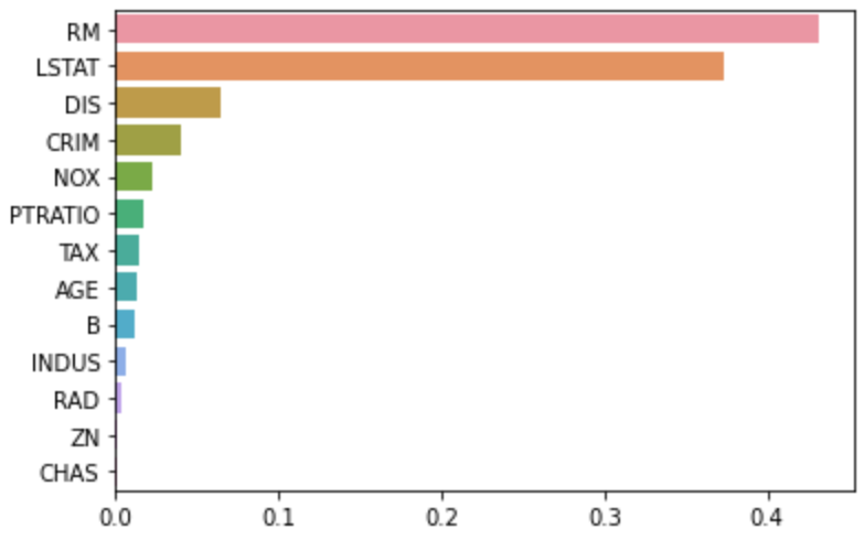
6. 트리회귀의 max_depth에 따른 오버피팅 확인해보기
트리회귀의 회귀 예측선을 그려보고 max_depth에 따른 오버피팅을 확인해보자
boston = load_boston()
bostonDF = pd.DataFrame(boston.data, columns = boston.feature_names)
bostonDF['PRICE'] = boston.target

print(bostonDF.shape)
bostonDF.head(3)
(506, 14)| CRIM | ZN | INDUS | CHAS | NOX | RM | AGE | DIS | RAD | TAX | PTRATIO | B | LSTAT | PRICE | |
|---|---|---|---|---|---|---|---|---|---|---|---|---|---|---|
| 0 | 0.00632 | 18.0 | 2.31 | 0.0 | 0.538 | 6.575 | 65.2 | 4.0900 | 1.0 | 296.0 | 15.3 | 396.90 | 4.98 | 24.0 |
| 1 | 0.02731 | 0.0 | 7.07 | 0.0 | 0.469 | 6.421 | 78.9 | 4.9671 | 2.0 | 242.0 | 17.8 | 396.90 | 9.14 | 21.6 |
| 2 | 0.02729 | 0.0 | 7.07 | 0.0 | 0.469 | 7.185 | 61.1 | 4.9671 | 2.0 | 242.0 | 17.8 | 392.83 | 4.03 | 34.7 |
import matplotlib.pyplot as plt
%matplotlib inline

# 한 개의 피처(RM)와 타겟값 선정
# x축:RM, y축:PRICE
bostonDF_sample = bostonDF[['RM','PRICE']]

# 데이터 중 100개만 샘플링
bostonDF_sample = bostonDF_sample.sample(n=100, random_state=0)

print(bostonDF_sample.shape)
plt.figure()
plt.scatter(bostonDF_sample.RM, bostonDF_sample.PRICE, c="darkorange")
(100, 2)
<matplotlib.collections.PathCollection at 0x7f8ae0f45390>
import numpy as np
from sklearn.linear_model import LinearRegression
from sklearn.tree import DecisionTreeRegressor

# 모델 : 선형회귀와 트리회귀
lr_reg = LinearRegression()
rf_reg2 = DecisionTreeRegressor(max_depth=2)
rf_reg7 = DecisionTreeRegressor(max_depth=7)

# x축 - 테스트 데이터를 4.5 ~ 8.5 범위, 100개 생성.
X_test = np.arange(4.5, 8.5, 0.04).reshape(-1, 1)

# 피처는 RM만, 타겟값 PRICE 추출
X_feature = bostonDF_sample['RM'].values.reshape(-1,1)
y_target = bostonDF_sample['PRICE'].values.reshape(-1,1)

# 학습
lr_reg.fit(X_feature, y_target)
rf_reg2.fit(X_feature, y_target)
rf_reg7.fit(X_feature, y_target)

# 예측
pred_lr = lr_reg.predict(X_test)
pred_rf2 = rf_reg2.predict(X_test)
pred_rf7 = rf_reg7.predict(X_test)
# 선형회귀와 트리회귀의 회귀 예측선 그리기 (X축 값 범위 4.5 ~ 8.5)
fig , (ax1, ax2, ax3) = plt.subplots(figsize=(14,4), ncols=3)
# 선형회귀
ax1.set_title('Linear Regression')
ax1.scatter(bostonDF_sample.RM, bostonDF_sample.PRICE, c="darkorange")
ax1.plot(X_test, pred_lr,label="linear", linewidth=2 )
# 트리회귀 max_depth=2
ax2.set_title('Decision Tree Regression: \n max_depth=2')
ax2.scatter(bostonDF_sample.RM, bostonDF_sample.PRICE, c="darkorange")
ax2.plot(X_test, pred_rf2, label="max_depth:3", linewidth=2)
# 트리회귀 max_depth=7 -> overfitting!
ax3.set_title('Decision Tree Regression: \n max_depth=7')
ax3.scatter(bostonDF_sample.RM, bostonDF_sample.PRICE, c="darkorange")
ax3.plot(X_test, pred_rf7, label="max_depth:7", linewidth=2)[<matplotlib.lines.Line2D at 0x7f8ae0fd5890>]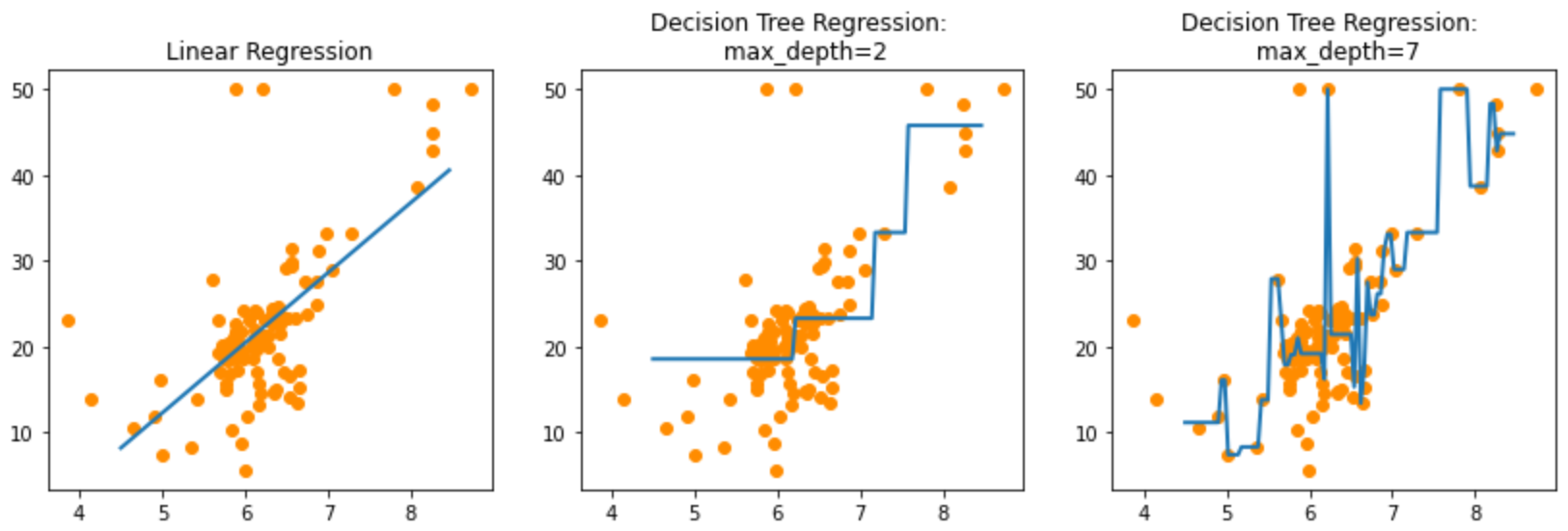
5.8절 끝

나무를 심는 사람