- 자료출처 : PyTorch로 시작하는 딥 러닝 입문
1. 다층 퍼셉트론으로 XOR 문제 풀기
# 파이토치에선 순전파와 역전파가 이 두줄의 코드로 구현가능
import torch
import torch.nn as nn
device = 'cuda' if torch.cuda.is_available() else 'cpu'
# for reproducibility
torch.manual_seed(777)
if device == 'cuda':
torch.cuda.manual_seed_all(777)# XOR 문제 정의
X = torch.FloatTensor([[0, 0], [0, 1], [1, 0], [1, 1]]).to(device)
Y = torch.FloatTensor([[0], [1], [1], [0]]).to(device)# 다층 퍼셉트론 설게 (은닉층이 3개인 인공신경망)
model = nn.Sequential(
nn.Linear(2, 10, bias=True), # input_layer = 2, hidden_layer1 = 10
nn.Sigmoid(),
nn.Linear(10, 10, bias=True), # hidden_layer1 = 10, hidden_layer2 = 10
nn.Sigmoid(),
nn.Linear(10, 10, bias=True), # hidden_layer2 = 10, hidden_layer3 = 10
nn.Sigmoid(),
nn.Linear(10, 1, bias=True), # hidden_layer3 = 10, output_layer = 1
nn.Sigmoid()
).to(device)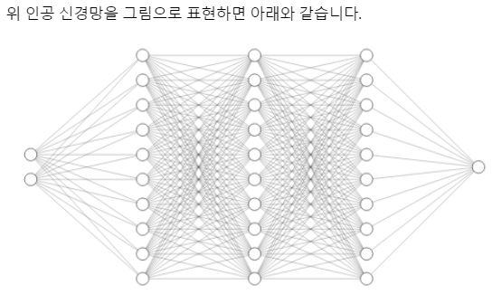
# 비용함수와 옵티마이저 선언
criterion = torch.nn.BCELoss().to(device) #크로스엔트로피 함수
optimizer = torch.optim.SGD(model.parameters(), lr=1)  # modified learning rate from 0.1 to 1
# 각 에포크마다 역전파 수행
for epoch in range(10001):
optimizer.zero_grad()
# forward 연산
hypothesis = model(X)
# 비용 함수
cost = criterion(hypothesis, Y)
cost.backward()
optimizer.step()
# 500의 배수에 해당되는 에포크마다 비용을 출력
if epoch % 500 == 0:
print(epoch, cost.item())0 0.7408947944641113
500 0.6931324601173401
1000 0.6931225061416626
1500 0.6931085586547852
2000 0.693087100982666
2500 0.6930486559867859
3000 0.6929655075073242
3500 0.6927102208137512
4000 0.6907041072845459
4500 0.007747023366391659
5000 0.0012943724868819118
5500 0.000667171785607934
6000 0.0004422826459631324
6500 0.0003283456608187407
7000 0.00026001702644862235
7500 0.0002146164479199797
8000 0.0001823932398110628
8500 0.00015838305989746004
9000 0.0001397983287461102
9500 0.00012501425226218998
10000 0.00011298747995169833#### 학습된 다층 퍼셉트론의 XOR 문제풀기with torch.no_grad():
hypothesis = model(X)
predicted = (hypothesis > 0.5).float()
accuracy = (predicted == Y).float().mean()
print('모델의 출력값(Hypothesis): ', hypothesis.detach().cpu().numpy())
print('모델의 예측값(Predicted): ', predicted.detach().cpu().numpy())
print('실제값(Y): ', Y.cpu().numpy())
print('정확도(Accuracy): ', accuracy.item())모델의 출력값(Hypothesis): [[6.8863672e-05]
[9.9988151e-01]
[9.9989235e-01]
[1.5687433e-04]]
모델의 예측값(Predicted): [[0.]
[1.]
[1.]
[0.]]
실제값(Y): [[0.]
[1.]
[1.]
[0.]]
정확도(Accuracy): 1.0- 예측값 0,1,1,0 과 실제값 0,1,1,0이 일치하는 것을 볼 수 있다.
2. 다층 퍼셉트론으로 MINST 분류하기
데이터 로드하기
import numpy as np
import matplotlib.pyplot as plt
%matplotlib inline
#사이킷런에서 제공하는 minst 데이터셋
from sklearn.datasets import fetch_openml
# 데이터셋 변수에 저장
mnist = fetch_openml('mnist_784', version=1, cache=True) mnist.data[0][150:200]array([ 0., 0., 3., 18., 18., 18., 126., 136., 175., 26., 166.,
255., 247., 127., 0., 0., 0., 0., 0., 0., 0., 0.,
0., 0., 0., 0., 30., 36., 94., 154., 170., 253., 253.,
253., 253., 253., 225., 172., 253., 242., 195., 64., 0., 0.,
0., 0., 0., 0., 0., 0.])mnist.target[0]'5'mnist.target = mnist.target.astype(np.int8)X = mnist.data / 255 # 0-255값을 [0,1] 구간으로 정규화
y = mnist.target훈련 데이터와 테스트 데이터의 분리
import torch
from torch.utils.data import TensorDataset, DataLoader
from sklearn.model_selection import train_test_splitX_train, X_test, y_train, y_test = train_test_split(X, y, test_size=1/7, random_state=0)
X_train = torch.Tensor(X_train)
X_test = torch.Tensor(X_test)
y_train = torch.LongTensor(y_train)
y_test = torch.LongTensor(y_test)
ds_train = TensorDataset(X_train, y_train)
ds_test = TensorDataset(X_test, y_test)
loader_train = DataLoader(ds_train, batch_size=64, shuffle=True)
loader_test = DataLoader(ds_test, batch_size=64, shuffle=False)다층 퍼셉트론
from torch import nn

model = nn.Sequential()
model.add_module('fc1', nn.Linear(28*28*1, 100))
# 시그모이드 대신 렐루를 썼다. 이유는 다음 포스팅에서.
model.add_module('relu1', nn.ReLU())
model.add_module('fc2', nn.Linear(100, 100))
model.add_module('relu2', nn.ReLU())
model.add_module('fc3', nn.Linear(100, 10))

print(model)
Sequential(
(fc1): Linear(in_features=784, out_features=100, bias=True)
(relu1): ReLU()
(fc2): Linear(in_features=100, out_features=100, bias=True)
(relu2): ReLU()
(fc3): Linear(in_features=100, out_features=10, bias=True)
)from torch import optim
# 오차함수 선택
loss_fn = nn.CrossEntropyLoss()
# 가중치를 학습하기 위한 최적화 기법 선택
optimizer = optim.Adam(model.parameters(), lr=0.01)def train(epoch):
model.train() # 신경망을 학습 모드로 전환
# 데이터로더에서 미니배치를 하나씩 꺼내 학습을 수행
for data, targets in loader_train:
optimizer.zero_grad() # 경사를 0으로 초기화
outputs = model(data) # 데이터를 입력하고 출력을 계산
loss = loss_fn(outputs, targets) # 출력과 훈련 데이터 정답 간의 오차를 계산
loss.backward() # 오차를 역전파 계산
optimizer.step() # 역전파 계산한 값으로 가중치를 수정
print("epoch{}:완료\n".format(epoch))def test():
model.eval() # 신경망을 추론 모드로 전환
correct = 0
# 데이터로더에서 미니배치를 하나씩 꺼내 추론을 수행
with torch.no_grad(): # 추론 과정에는 미분이 필요없음
for data, targets in loader_test:
outputs = model(data) # 데이터를 입력하고 출력을 계산
# 추론 계산
_, predicted = torch.max(outputs.data, 1) # 확률이 가장 높은 레이블이 무엇인지 계산
correct += predicted.eq(targets.data.view_as(predicted)).sum() # 정답과 일치한 경우 정답 카운트를 증가
# 정확도 출력
data_num = len(loader_test.dataset) # 데이터 총 건수
print('\n테스트 데이터에서 예측 정확도: {}/{} ({:.0f}%)\n'.format(correct,
data_num, 100. * correct / data_num))for epoch in range(3):
train(epoch)
test()epoch0:완료
epoch1:완료
epoch2:완료
테스트 데이터에서 예측 정확도: 9542/10000 (95%)
index = 2018

model.eval()  # 신경망을 추론 모드로 전환
data = X_test[index]
output = model(data)  # 데이터를 입력하고 출력을 계산
_, predicted = torch.max(output.data, 0)  # 확률이 가장 높은 레이블이 무엇인지 계산

print("예측 결과 : {}".format(predicted))

X_test_show = (X_test[index]).numpy()
plt.imshow(X_test_show.reshape(28, 28), cmap='gray')
print("이 이미지 데이터의 정답 레이블은 {:.0f}입니다".format(y_test[index]))
예측 결과 : 2
이 이미지 데이터의 정답 레이블은 2입니다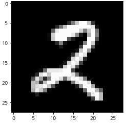

나무를 심는 사람