[작성자 : 권오현]
Intro
Real-World, 많은 Large Graphs가 존재한다. Recommendation Systems(ex. Amazon, Youtube, Pinterest, etc.) , Heterogeneous Graphs(MS Academic graph), Social Networks(ex. Facebook, Twitter, Instagram), Machine Learning Task (ex. Paper categorization, Author Collaboration, Paper citation recommendation), Knowledge Graph(ex. Wikidata, Freebase)
Motivate : How we do scale up GNN's to graphs of size (100M to 100B)?
-
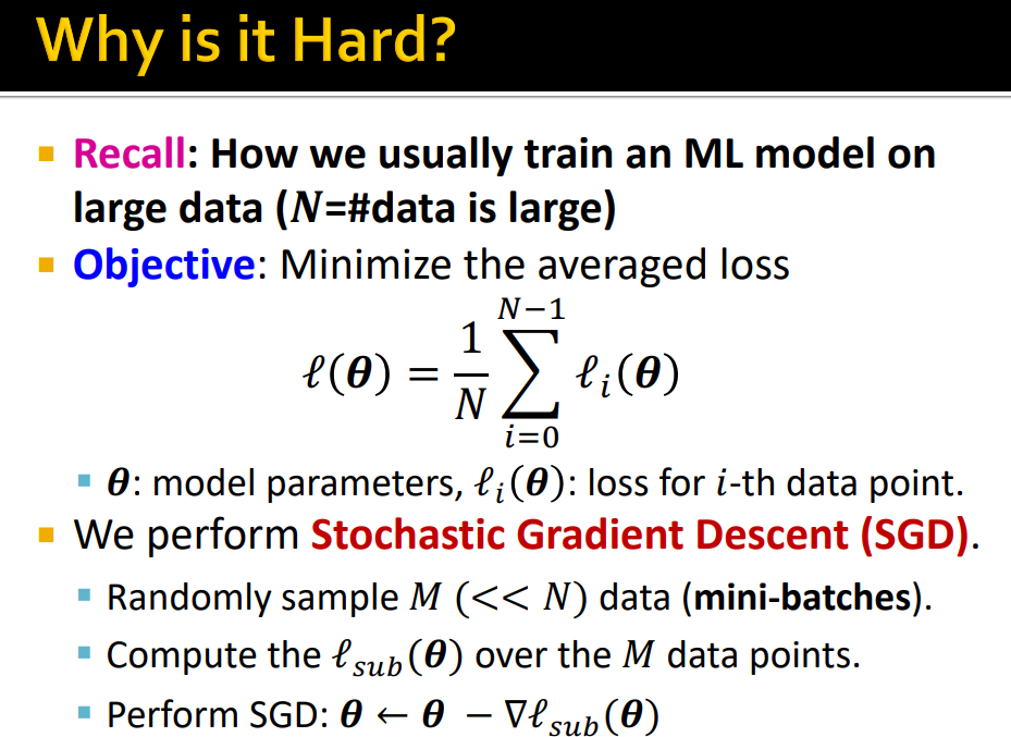
기존 DL training을 생각해 보면 Loss를 통해 model parameters update
-
data가 크기 때문에 mini-batches를 통해 학습 (Node level prediction task - subsample a set of node N)
-
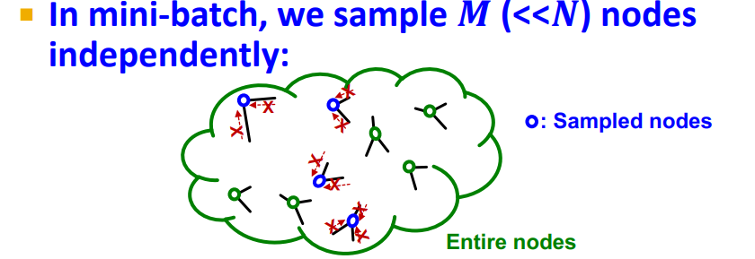
Graph Neural Networks에서 mini-batch는 independently sampling, 대부분 neighbors의 information을 aggregating하지 못함
-
Full-batch의 경우 모든 nodes의 embedding을 동시에 생성한다는 문제점이 있다. (graph는 각각의 layer에서 all node embedding을 계산해야 한다. 이 때 이전 layer의 all node embedding을 사용하여 다음 layer의 embedding을 계산하게 됨) -> recursive structure이기 때문에 memory가 상당히 요구됨
-
Full-batch의 경우 Time wise, GPU Memory limited로 인해 학습이 불가능 하다.
-
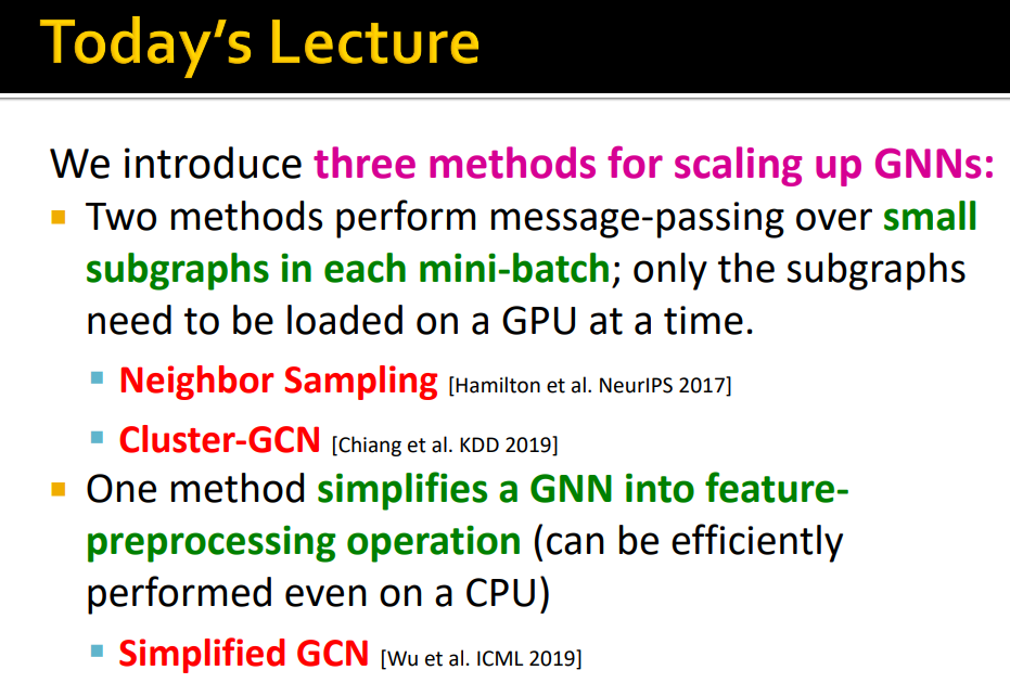
Scaling up GNNs을 학습하는 3가지 방법을 제안한다.
-
small subgraphs의 message-passing을 통한 방법, Simplified GNN
Neighbor Sampling
Main Idea : GraphSAGE의 방법을 통해 graph를 mini-batch로 학습할 수 있게 함
-
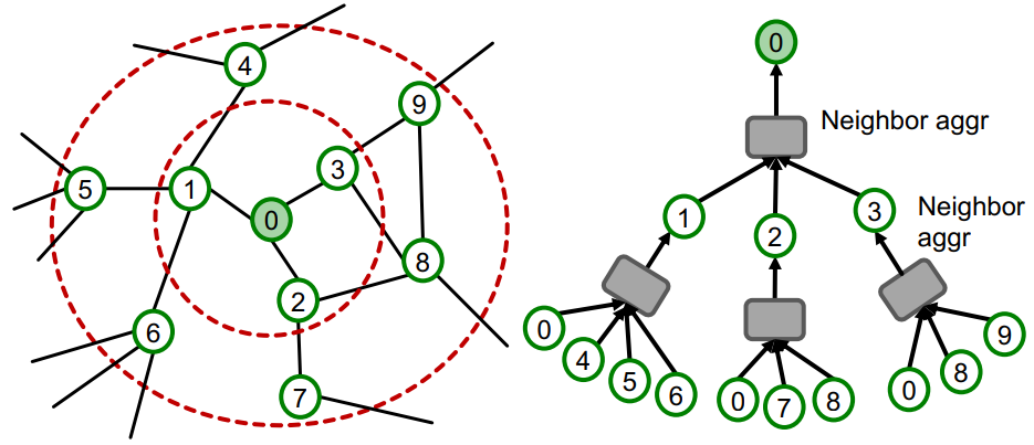
GNN은 neighborhood aggregation을 통해 node embedding을 생성한다. (Message Passing을 통해 Computation graph 생성)
-
Node 0의 embedding을 구하기 위해서 Graph Structure, Two-Hop neighborhood node feature가 필요함
-
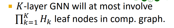
K-layer GNN의 경우 K-hop neighborhood와 features를 통해 embedding을 generate(= K-hop neighborhood의 embedding을 알면 embedding을 generate)
-
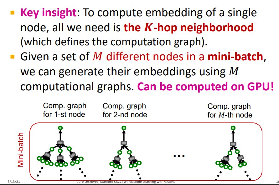
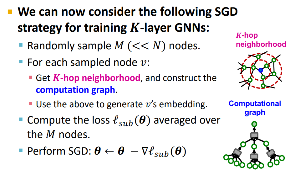
Main Insight : Single Node의 embedding을 계산하기 위해 K-hop neighborhood가 필요하다. Node Embedding이 아닌 K-hop neighborhoods 기반의 Computation graph를 통해 Mini-batch로 학습을 할 수 있다.
-
M개의 sample에 대해서 K-hop neighborhood를 통해 Gradient를 계산하여 학습
-
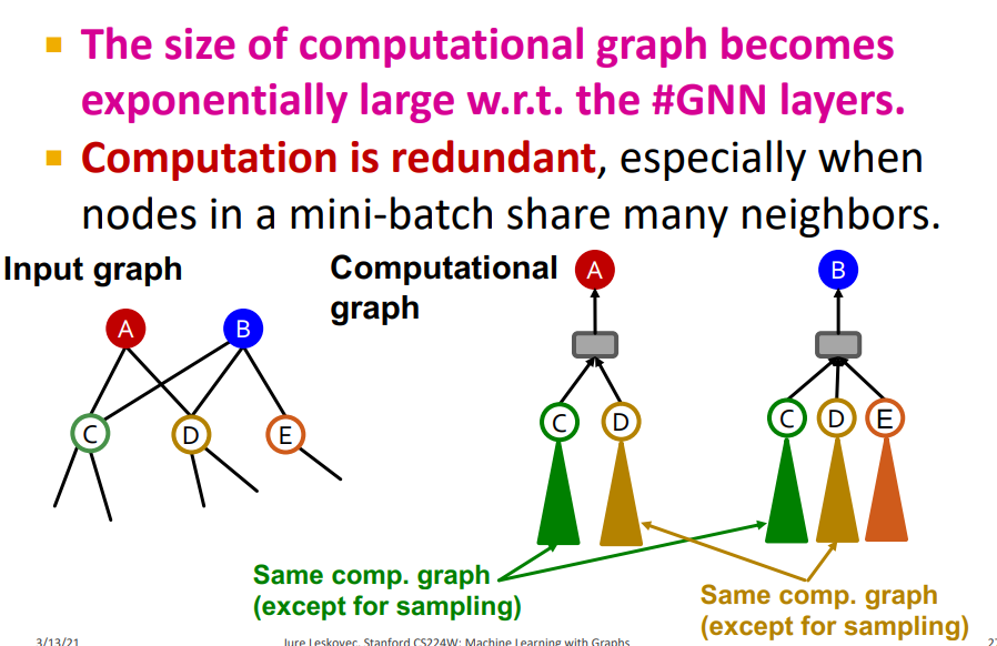
전체 K-hop neigborhood의 computation graph를 구해서 one node embedding을 구해야 하기 때문에 매우 expensive하다.
- Computation Graph는 Exponential하게 커진다.
- Natural graphs에서 hub-nodes(high-degree nodes, celebrity nodes)가 존재하기 때문에 expensive 하다
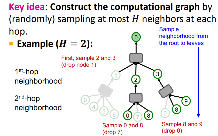
- 이를 해결하기 위해 neighbor sampling을 제안한다
- 모든 Node, layer에서 H random neighbors를 뽑는다 (computation graph는 exponential하게 증가하지만, Upper bounded by H)
Remarks on Neighbor sampling
-
Trade off in sampling Number H : H가 작으면 Neighbor aggregation에 효과적이지만 entire subpart of network를 고려하지 않아 variance가 커져 unstable learning하게 된다
-
Computation Time : Computational graph는 Exponential하게 증가하는데 H가 크지 않으면 K의 관점에서 깊게 학습하는게 아니다.
-
How to sample the nodes : Uniformly하게 H neighbors를 sampling 한다. Real-world networks에서는 highly skewed degree distribution을 가지고 있기 때문에 Important neighbors가 sampling 되지 않고 Noisy하게 될 수 있다.
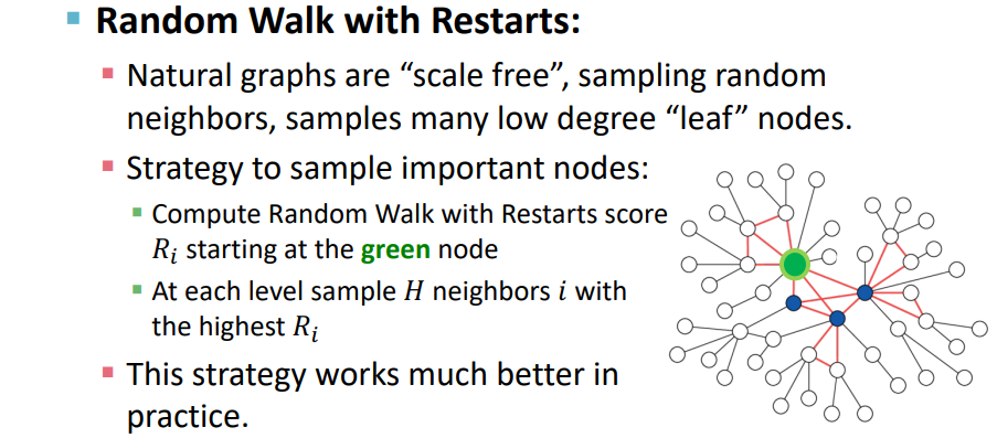
이를 해결하기 위해 Random walk를 적용하여 nodes를 sampling 한다.
Issues with Neighbor Sampling
-
Neighbor sampling, computational graph는 computational efficency 하지만 computational graphs는 여전히 크다. (GNN는 message-passing layers가 많이 있기 때문에)
-
Computation is redundant 이를 해결하기 위해 Same components를 except(HAGs), Cluster-GCN
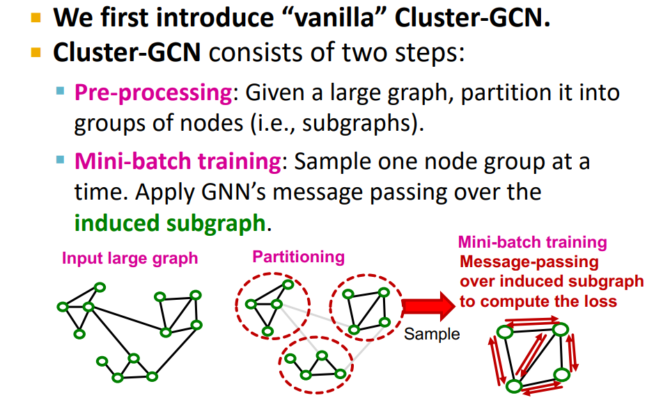
Cluster-GCN
-
Cluster-GCN은 Full-batch에서 Motivate되었다.
-
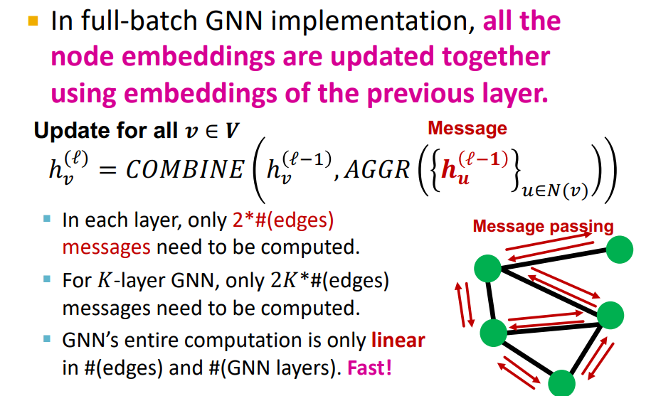
Full-batch training은 L-1의 모든 nodes embedding을 통해 L layer의 embedding을 계산한다. (각각의 layer에서 2K*# 의 message가 compute되어야 함, GNN's computation은 linear하지만, Graph가 매우 크기 때문에 한번에 계산 못한다.)
-
Full-batch의 경우 Layer-wise node embedding update를 하기 때문에 previous layer의 embedding을 re-use하게 해줌 (computational redundancy를 줄일 수 있다.)
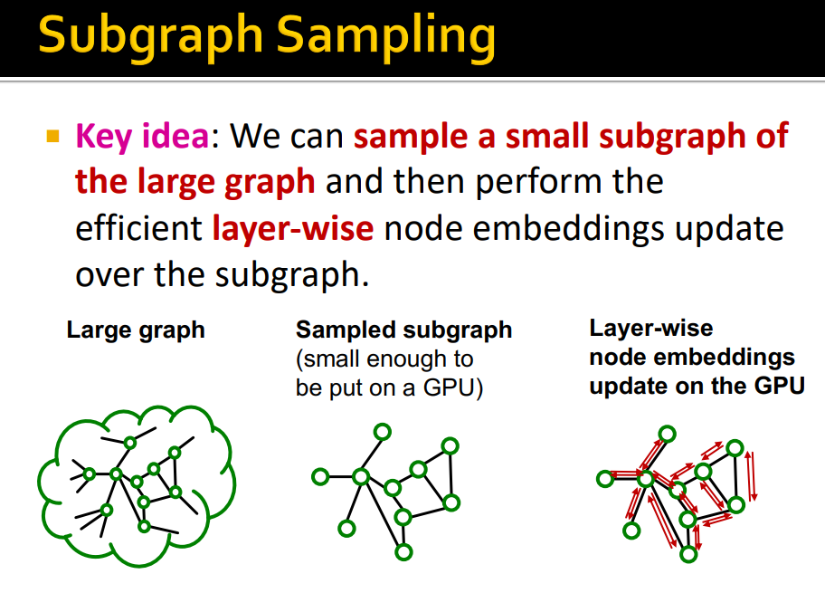
- Cluster-GCN Key Idea : 전체 graph를 small sub-parts로 나누어 subgraphs를 통해 full-batch implementation 수행
vs Neighbor sampling : Compute the computation graph for each individual node and entire graph -> Subgraph Sampling
-
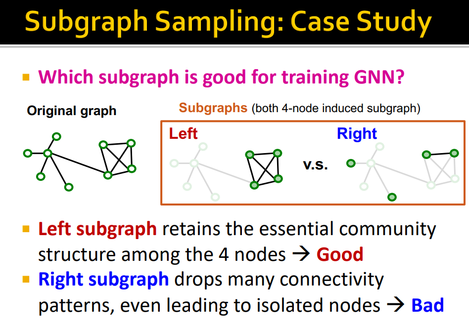
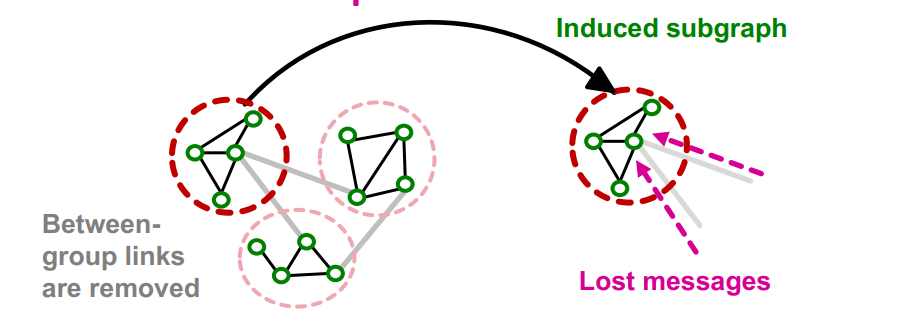
GNN training에 좋은 Subgraph는 어떤 것인가 ? Original Graph의 edges를 가능한 많이 retain한 subgraph
-
Real world graph에는 community structure, clustering이 존재하기 때문에 community structure를 잘 보존하는 것이다.
-
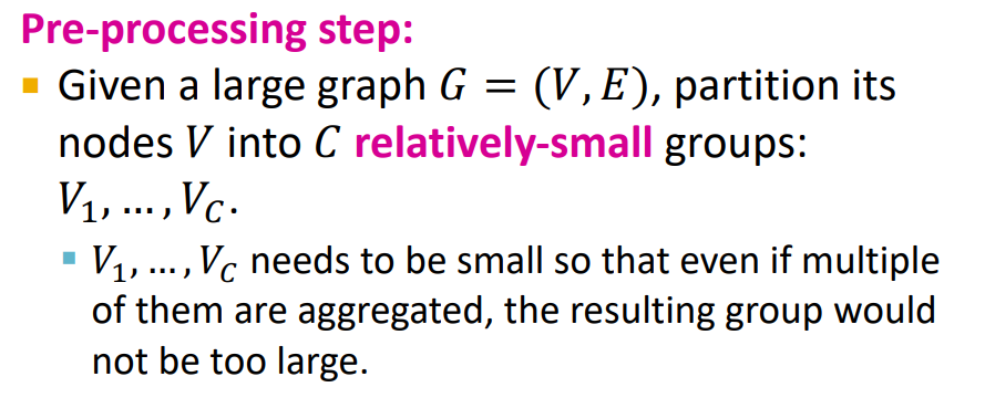
Pre-processing : Original graph partitioning
- Louvain, METIS, BigCLAM을 통해 Community detection, edge drop
-
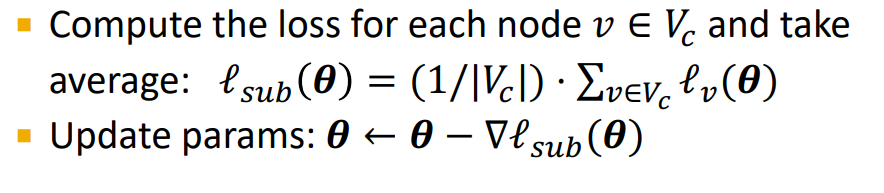
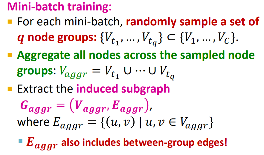
Mini-batch training : Sample one node group, perform full batch message passing over that entire subgraph, compute subgraph's node embedding and loss
GraphSAGE vs Cluster-GCN : neighborhood sampling( can be distributed across the entire network) vs Neighborhood sampling(just being limited to the subgraph we sample)
Problem
-
Induced subgraphs는 links를 drop하기 때문에 다른 group에서 message를 받지 못하는 문제점이 있다.
-
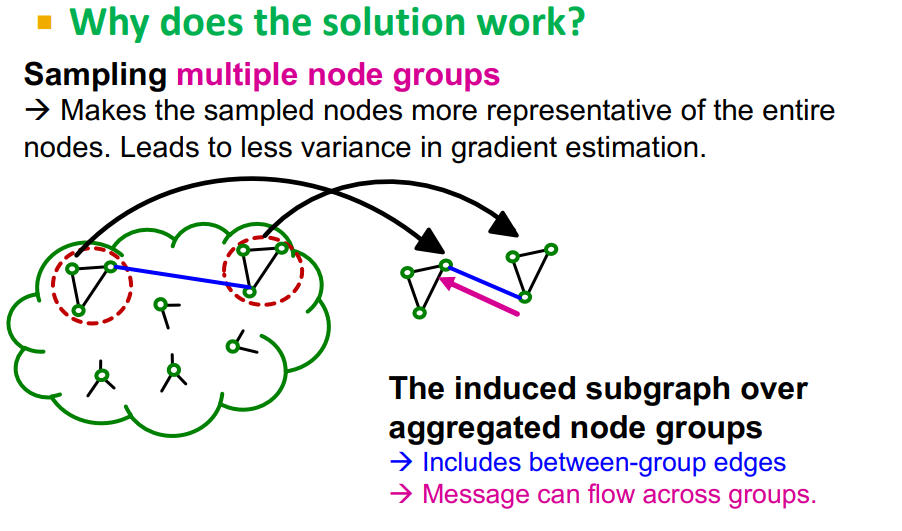
Graph community detection은 similar nodes를 group으로 묶기 때문에, sample node group은 전체 group에서 일부분만 고려한다. Fluctuates a lot from a node group to another(= gradient high variance, slow convergence of SGD)
-
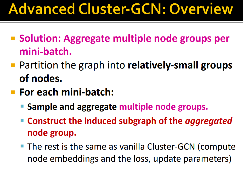
이를 해결하기 위해 Advanced Cluster-GCN이 제안됨
Advanced Cluster-GCN
-
Graph Partitioning을 더 작게 하여 mini-batch training에서 multiple node group을 aggregate한다.
-
Induced subgraph를 multiple node group으로 구성하여 결과적으로 more diverse하게 학습을 한다.
Training
Vanilla Cluster-GCN과 동일하게 학습
Comparision
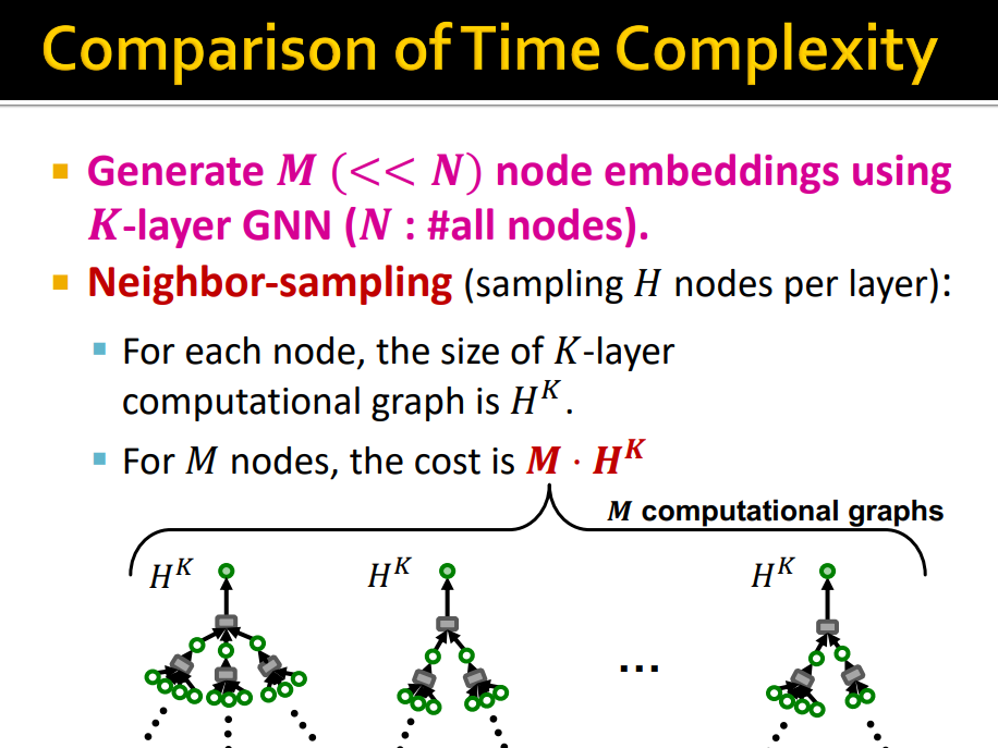
- Neighbor-sampling은 각 node 마다 H개 sampling 하기 때문에 computational graph의 cost는 , M nodes에 대해서는
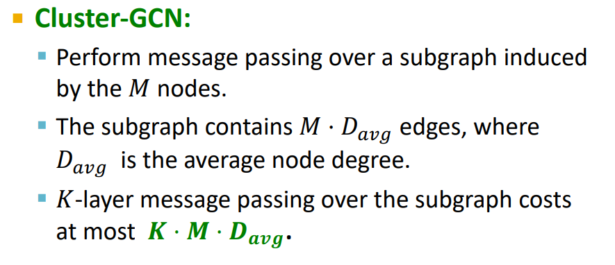
- Cluster-GCN은 M nodes에 대해 induced graph를 통해 message passing을 하기 때문에 의 cost를 가진다
-
Cluster-GCN이 Linear하게 증가하기 때문에 더욱 효율적이다. 하지만 layer K가 크지 않으면 neighbor-sampling이 더 많이 사용된다.
-
Cluster-GCN은 community간의 edges를 drop하기 때문에 biased gradient estimates를 구할 가능성이 있다
Simplifying GCN
-
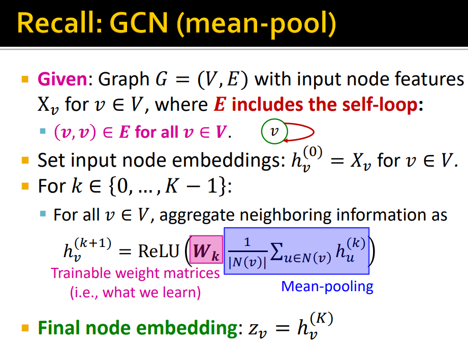
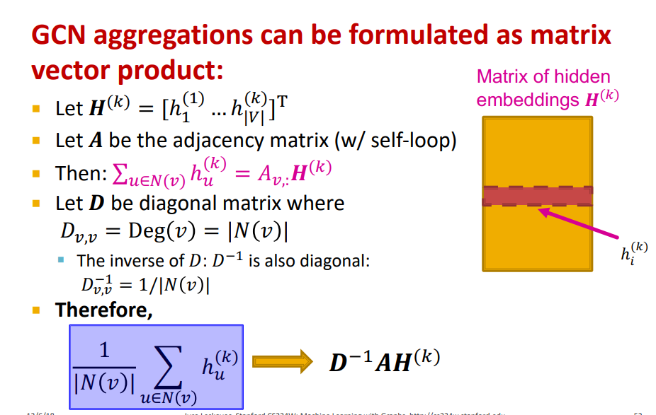
GCN은 Node features를 input으로 하여 K+1 layer의 embedding을 K layer의 neighborhood의 embedding layer와 Trainable weight, activation function을 통해 구한다.
-
위의 식을 Matrix Form으로 정의할 수 있다 (Adjacency Matrix와 embedding Matrix의 product)
-
= Diagonal Matrix(Neighborhood degree)
-
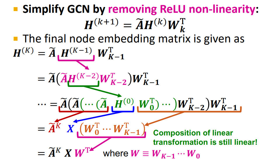
Simplify GCN은 이러한 식에서 non-linearity를 제거한 방법이다
-
: connects the target node to its neighbors, neighbors of neighbors(= one-hop father out in the network as we increase)
-
: node features
-
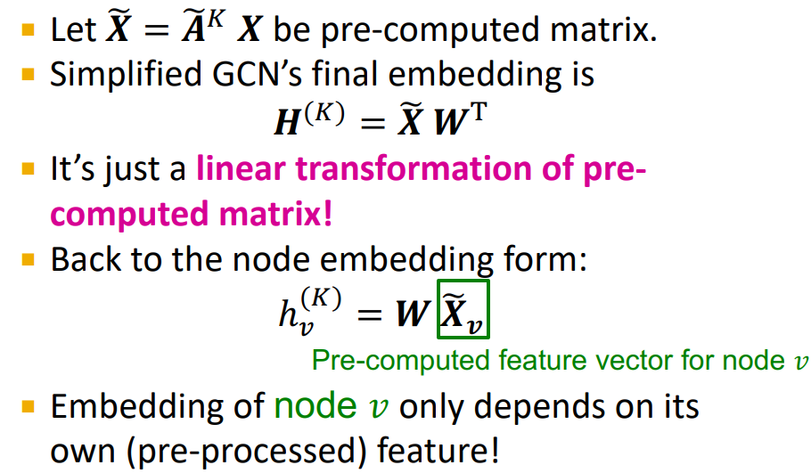
, 는 learnable parameters가 아니기 때문에 pre-computed하여 더욱 efficiently (sequene of sparse matrix vector products)
-
pre-computed matrix Linear transformation으로 embedding을 구할 수 있음
-
node v의 embedding은 pre-computed된 feature에만 의존하게 된다.
-
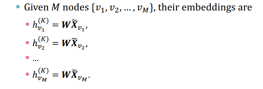
의 row를 sampling하여 mini-batch training 가능
-
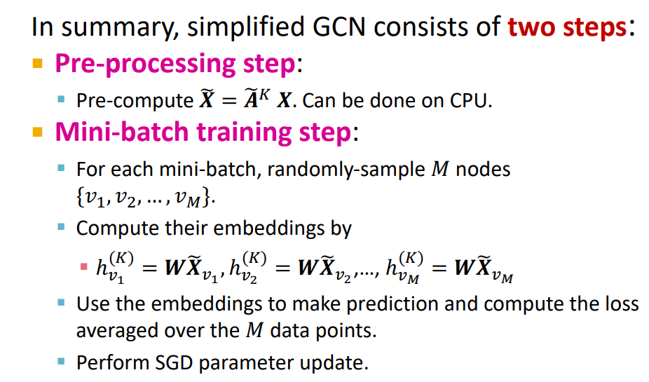
Simpified GCN은 Two steps 로 구성되어 있다.
-
Pre-processing Step : 는 neighborhood의 degree, 는 node features
-
Mini-batch training step : 의 row가 random sample
- 장점 : Embedding of every node computation of it's independent from the other nodes
Comparision with Other Methods
-
Neighbor sampling과 비교하여 Simplified GCN은 computatioal graph를 구할 필요가 없고 학습이 쉽다.
-
Cluster-GCN은 Multiple Group에서 sampling 하여 연산을 하였지만, Simplified GCN은 Entire of nodes에서 random sampling 하면 된다.
-
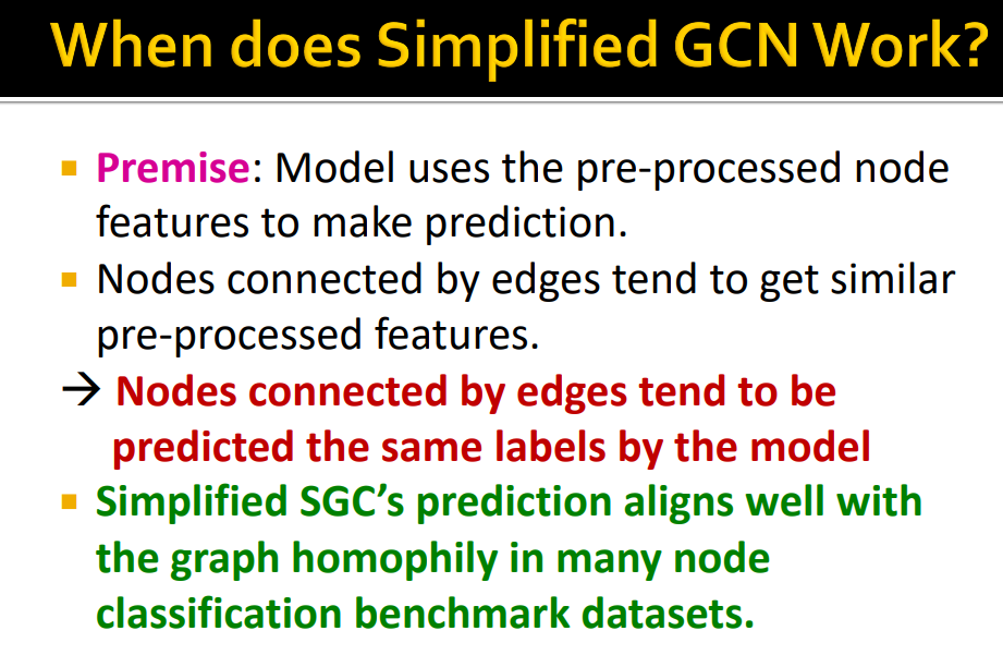
하지만 Original GNN과 비교하여 non-lineartiy를 제거 했기 때문에 expressive power는 제한된다.
-
그럼에도 불구하고 Real-world cases에서 잘 작동하고 Original GNN 보다 조금 안좋을 뿐이다.
-
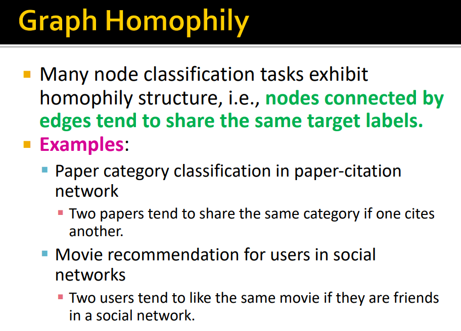
Graph에는 Homophily가 존재하기 때문이다.
-
Pre-processed feature는 neighboring node features를 iterative하게 averaging 하기 때문에 Node Classification에서 Simplified GCN이 작동이 잘된다.
-
Pre-processed feature는 neighboring node features를 iterative하게 averaging 하기 때문에 잘 작동한다.