h1n1 vaccination classification
Feature 설명
-
behavioral_antiviral_meds - 항바이러스제를 복용했습니다. (이진)
-
behavioral_avoidance - 독감 같은 증상을 가진 다른 사람들과의 긴밀한 접촉을 피했습니다. (이진)
-
behavioral_face_mask - 페이스 마스크를 구입했습니다. (이진)
-
behavioral_wash_hands - 손을 자주 씻거나 손 세정제를 사용했습니다. (이진)
-
behavalion_large_garings - 큰 모임에서 시간이 단축되었습니다. (이진)
-
behavioral_outside_home - 자신의 가정 이외의 사람들과의 접촉이 감소하였다. (이진)
-
bevehaval_touch_face - 눈, 코, 입의 접촉을 피했습니다. (이진)
-
doctor_recc_h1n1 - H1N1 독감백신은 의사가 권장하였다. (이진)
-
doctor_recc_seasonal - 계절 독감 백신은 의사가 권장하였다. (이진)
-
chronic_med_condition - 천식 또는 다른 폐 질환, 당뇨병, 심장 질환, 신장 질환, 겸상적혈구 빈혈 또는 기타 빈혈, 신경성 또는 신경근육 질환, 간 질환 또는 만성 질환 또는 만성 질환에 의해 복용된 약화된 면역 체계를 가지고 있다. 병. (병)
-
child_under_6_months - 생후 6개월 미만 아동과 정기적으로 밀접하게 접촉합니다. (이진)
-
health_insurance - 건강보험이 있습니다. (이진)
-
health_worker - 의료 종사자입니다. (이진)
-
opinion_h1n1_vacc_effective - H1N1 백신 효과에 대한 응답자의 의견. 전혀 효과적이지 않다; 매우 효과적이지 않다; 잘 모른다; 다소 효과적이다; 매우 효과적이다.
-
opinion_h1n1_risk - 백신 없이 H1N1 독감에 걸릴 위험에 대한 응답자의 의견. 매우 낮음, 다소 낮음, 잘모름, 다소 높음, 매우 높음
-
opinion_h1n1_sick_from_vacc - H1N1 백신을 복용하여 병에 걸리는 것에 대한 응답자의 걱정. 전혀 걱정 안 해. 별로 걱정 안 해. 몰라. 어느 정도 걱정해. 아주 걱정해.
-
opinion_seas_vacc_effective - 계절 독감 백신 효과에 대한 응답자의 의견. 전혀 효과적이지 않다; 매우 효과적이지 않다; 잘 모른다; 다소 효과적이다; 매우 효과적이다.
-
opinion_sea_risk - 백신 없이 계절성 독감에 걸릴 위험에 대한 응답자의 의견. 매우 낮음, 다소 낮음, 잘모름, 다소 높음, 매우 높음
-
opinion_sea_sick_from_vacc - 계절성 독감 백신을 복용하여 병에 걸리는 것에 대한 응답자들의 걱정. 전혀 걱정 안 해. 별로 걱정 안 해. 몰라. 어느 정도 걱정해. 아주 걱정해.
-
agegrp - 응답자 연령 그룹. 6개월 - 9년, 10 - 17년, 18 - 34년, 35 - 44년, 45 - 54년, 55 - 64년, 65년 이상
-
education_comp - 자체 보고된 교육 수준입니다.
1 = = 12년, 2 = 12년, 3 = 일부 대학, 4 = 대학 졸업 -
raceeth4_i - 응답자 레이스
1 = 히스패닉, 2 = 비히스패닉, 흑인 전용, 3 = 비히스패닉, 백인 전용, 4 = 비히스패닉, 기타 또는 다중 인종 -
sex_i - 응답자의 성별.
1 = 남성, 2 = 여성 2 -
inc_pov - 2008년 인구조사 빈곤 문턱에 대한 응답자의 가구 연간 소득.
1 = = 75,000달러, 2 = = 75,000달러, 3 = 빈곤 이하, 4 = 미상 -
marital - 응답자의 혼인 여부.
1 = 결혼, 2 = 결혼하지 않음 -
rent_own_r - 응답자의 주거 상황.
1 = 자택 소유, 2 = 자택 임대 또는 기타 약정 -
employment_status - 응답자의 고용상태입니다.
고용; 노동력이 아님; 실업자 -
census_region - 거주 지역의 참 인구 조사 지역(1=178; 2=198; 3=남쪽, 4=서쪽)
-
census_msa - 미국 인구조사에 의해 정의된 대로 응답자가 대도시 통계 지역(MSA) 내에 거주하는 경우.
-
n_adult_r - 가구의 기타 성인 수.
-
household_children - 가구의 자녀 수입니다.
-
n_people_r - 가구의 성인 수.
-
employment_industry - 산업 응답자 유형을 에 고용합니다.
-
employment_occupation - 응답자 직업 유형. 값은 짧은 임의 문자열로 표시됩니다.
-
hhs_region - HHS 감시 지역 번호
Region 1: CT,ME,MA,NH,RI,VT
Region 2: NJ,NY
Region 3: DE, DC, MD, PA, VA,WV
Region 4: AL, FL, GA, KY, MS, NC, SC,TN
Region 5: IL, IN, MI, MN, OH,WI
Region 6: AR, LA, NM, OK, TX
Region 7: IA,KS,MO,NE
Region 8: CO, MT, ND, SD, UT, WY
Region 9: AZ, CA, HI, NV
Region 10: AK, ID, OR, WA -
state - 거주 상태
라이브러리 불러오기
# !pip install category_encoders

import numpy as np
import pandas as pd

import matplotlib.pyplot as plt
import seaborn as sns

from sklearn.model_selection import train_test_split, GridSearchCV
from category_encoders import OrdinalEncoder
from sklearn.ensemble import RandomForestClassifier
from sklearn.impute import SimpleImputer
from sklearn.pipeline import make_pipeline
from sklearn.metrics import f1_score, accuracy_score, plot_confusion_matrix
from sklearn.preprocessing import LabelEncoder, PolynomialFeatures
from sklearn.linear_model import LogisticRegression
from sklearn.tree import DecisionTreeClassifier

from tqdm.notebook import tqdm

import warnings
warnings.filterwarnings('ignore')
데이터 생성
target = 'vacc_h1n1_f'
train = pd.merge(pd.read_csv('https://ds-lecture-data.s3.ap-northeast-2.amazonaws.com/vacc_flu/train.csv'),
                 pd.read_csv('https://ds-lecture-data.s3.ap-northeast-2.amazonaws.com/vacc_flu/train_labels.csv')[target], left_index=True, right_index=True)
test = pd.read_csv('https://ds-lecture-data.s3.ap-northeast-2.amazonaws.com/vacc_flu/test.csv')
sample_submission = pd.read_csv('https://ds-lecture-data.s3.ap-northeast-2.amazonaws.com/vacc_flu/submission.csv')


#train, validation 분리
train, val = train_test_split(train, test_size = 0.2, stratify = train[target], random_state = 2) #stratify : 원래 class의 비율을 유지시켜줌

train.shape, val.shape, test.shape
EDA 및 전처리
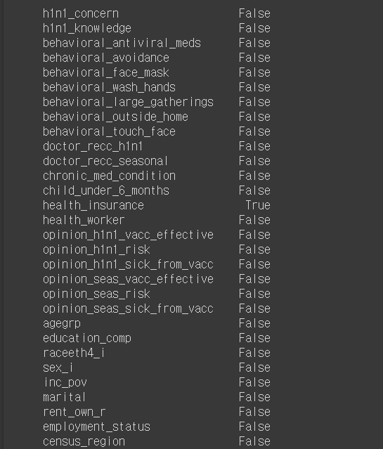
# na 비율이 30% 이상인 feature 찾기
train.isna().sum()/len(train) > 0.3
#na처리
from sklearn.preprocessing import LabelEncoder

encoder = LabelEncoder()

def pre_na(df):
    cols = list(df.columns)

    for col in cols:
        if df[col].dtype == int or df[col].dtype == float:
            df[col].fillna(value = df[col].mean(), inplace = True)
        else:
            df[col].fillna(value = 'X', inplace = True)

        df[col] = encoder.fit_transform(df[col])

    return df

train = pre_na(train)
val = pre_na(val)
test = pre_na(test)
#분포확인#분포확인
cols = list(train.columns)
plt.figure(figsize = (20, 10))
for i, col in enumerate(cols):
plt.subplot(6,7,i+1)
try:
sns.distplot(train[col])
except:
pass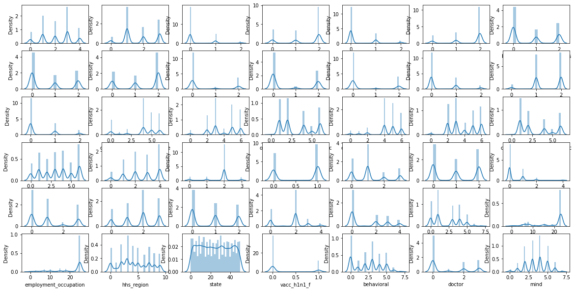
#correlation 확인
plt.figure(figsize = (10,10))

sns.heatmap(train.corr()[['vacc_h1n1_f']].sort_values('vacc_h1n1_f', ascending = False));
Feature engineering
# feature engineering

def engineer(df):

    #높은 카디널리티 제거
    # labels = df.nunique()

    # selected_features = labels[labels < 20].index.tolist()
    # df = df[selected_features]

    cols = list(df.columns)

    behavioral = []

    for col in cols:
        if 'behavioral' in col:
            behavioral.append(col)

    #예방 행위
    df['behavioral'] = df[behavioral].sum(axis = 1)

    #의사소견
    df['doctor'] = df['doctor_recc_h1n1'] + df['doctor_recc_seasonal']

    #경각심
    df['mind'] = df['health_worker'] + df['h1n1_knowledge'] + df['h1n1_concern']

    #NA 비율이 높은 columns 삭제
    # df.drop(['health_insurance','employment_industry','employment_occupation'],axis=1)

    return df

train = engineer(train)
val = engineer(val)

#중복제거
train.drop_duplicates(inplace = True)
val.drop_duplicates(inplace = True)

test = engineer(test)

list(train.columns)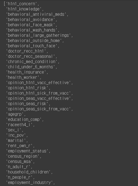
# class 분리

features = train.drop(target, axis = 1).columns

X_train = train[features]
y_train = train[target]

X_val = val[features]
y_val = val[target]

X_train_val = pd.concat([X_train, X_val])
y_train_val = pd.concat([y_train, y_val])

X_test = test[features]
모델링
#파라미터 튜닝 준비

pipe_temp = make_pipeline(
    OrdinalEncoder(),
    SimpleImputer(),
    PolynomialFeatures(2)
)

X_train_val2 = pipe_temp.fit_transform(X_train_val)
X_test2 = pipe_temp.transform(X_test)
X_train2 = pipe_temp.transform(X_train)
X_val2 = pipe_temp.transform(X_val)
#feature
poly = pipe_temp.named_steps['polynomialfeatures']
len(poly.get_feature_names(X_train_val.columns))903
#중요 feature 90개 생성

from sklearn.feature_selection import SelectKBest

selector = SelectKBest(k = 90)

X_train_val_selected = selector.fit_transform(X_train_val2, y_train_val)
X_test_selected = selector.transform(X_test2)
X_train_selected = selector.transform(X_train2)
X_val_selected = selector.transform(X_val2)

mark = selector.get_support()

all_names = pd.DataFrame(poly.get_feature_names(X_train_val.columns))
select_names = all_names[mark]
# 중요 90개의 feature를 가지는 형태로 데이터 변환
# make_pipeline을 통해서 더 간편하게 설정할 수 있음
X_train_val = pd.DataFrame(X_train_val_selected, columns = select_names[0])
X_test = pd.DataFrame(X_test_selected, columns = select_names[0])
X_train = pd.DataFrame(X_train_selected, columns = select_names[0])
X_val = pd.DataFrame(X_val_selected, columns = select_names[0])#best parameter 찾기
param_grid = {
'max_features' : ['sqrt', 0.25, 0.5],
'max_depth' : [10, 20, 30, None]
}
grid = GridSearchCV(RandomForestClassifier(n_jobs = -1, n_estimators=200), param_grid, cv = 5, verbose = 1)
grid.fit(X_train_val, y_train_val)
print('best parameters : \n', grid.best_params_)
print('best score : ', grid.best_score_)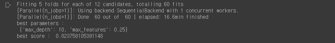
#최적의 파라미터들을 선정하여 모델링
%%time

pipe = make_pipeline(
    OrdinalEncoder(),
    SimpleImputer(),
    PolynomialFeatures(2),
    RandomForestClassifier(n_jobs = -1, random_state = 10, n_estimators = 200, max_depth = 10 , max_features = 0.25, oob_score = True)
)

pipe.fit(X_train_val, y_train_val)print('Training accuracy : ', pipe.score(X_train, y_train))
print('Validation accuracy : ', pipe.score(X_val,y_val))
y_pred = pipe.predict(X_val)
print('Validation F1 score : ', f1_score(y_val, y_pred))
#예측 결과 확인
#confusion matrix

from sklearn.metrics import classification_report, confusion_matrix

pcm = plot_confusion_matrix(
    pipe,
    X_val,
    y_val,
    cmap = 'Blues'
)
plt.title('Confusion matrix, Threshold : 0.5')
plt.show()

threshold = [0.1, 0.2, 0.3, 0.4, 0.5, 0.6, 0.7, 0.8, 0.9]

for thr in threshold:
    print('threshold : ', thr)

    y_pred_proba = pipe.predict_proba(X_val)[:,1]
    y_pred = (y_pred_proba > thr)

    con = confusion_matrix(
        y_val,
        y_pred
    )
    print('confusion matrix : \n',con)
    print()
    print(classification_report(y_val, y_pred))
    print()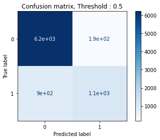
threshold : 0.1
confusion matrix :
[[3213 3194][ 137 1873]]
          precision    recall  f1-score   support

       0       0.96      0.50      0.66      6407
       1       0.37      0.93      0.53      2010

accuracy                           0.60      8417
macro avg 0.66 0.72 0.59 8417
weighted avg 0.82 0.60 0.63 8417
threshold : 0.2
confusion matrix :
[[4860 1547][ 401 1609]]
          precision    recall  f1-score   support

       0       0.92      0.76      0.83      6407
       1       0.51      0.80      0.62      2010

accuracy                           0.77      8417
macro avg 0.72 0.78 0.73 8417
weighted avg 0.82 0.77 0.78 8417
threshold : 0.3
confusion matrix :
[[5648 759][ 600 1410]]
          precision    recall  f1-score   support

       0       0.90      0.88      0.89      6407
       1       0.65      0.70      0.67      2010

accuracy                           0.84      8417
macro avg 0.78 0.79 0.78 8417
weighted avg 0.84 0.84 0.84 8417
threshold : 0.4
confusion matrix :
[[5986 421][ 731 1279]]
          precision    recall  f1-score   support

       0       0.89      0.93      0.91      6407
       1       0.75      0.64      0.69      2010

accuracy                           0.86      8417
macro avg 0.82 0.79 0.80 8417
weighted avg 0.86 0.86 0.86 8417
threshold : 0.5
confusion matrix :
[[6215 192][ 904 1106]]
          precision    recall  f1-score   support

       0       0.87      0.97      0.92      6407
       1       0.85      0.55      0.67      2010

accuracy                           0.87      8417
macro avg 0.86 0.76 0.79 8417
weighted avg 0.87 0.87 0.86 8417
threshold : 0.6
confusion matrix :
[[6306 101][1084 926]]
          precision    recall  f1-score   support

       0       0.85      0.98      0.91      6407
       1       0.90      0.46      0.61      2010

accuracy                           0.86      8417
macro avg 0.88 0.72 0.76 8417
weighted avg 0.86 0.86 0.84 8417
threshold : 0.7
confusion matrix :
[[6357 50][1249 761]]
          precision    recall  f1-score   support

       0       0.84      0.99      0.91      6407
       1       0.94      0.38      0.54      2010

accuracy                           0.85      8417
macro avg 0.89 0.69 0.72 8417
weighted avg 0.86 0.85 0.82 8417
threshold : 0.8
confusion matrix :
[[6399 8][1535 475]]
          precision    recall  f1-score   support

       0       0.81      1.00      0.89      6407
       1       0.98      0.24      0.38      2010

accuracy                           0.82      8417
macro avg 0.89 0.62 0.64 8417
weighted avg 0.85 0.82 0.77 8417
threshold : 0.9
confusion matrix :
[[6407 0][1889 121]]
          precision    recall  f1-score   support

       0       0.77      1.00      0.87      6407
       1       1.00      0.06      0.11      2010

accuracy                           0.78      8417
macro avg 0.89 0.53 0.49 8417
weighted avg 0.83 0.78 0.69 8417
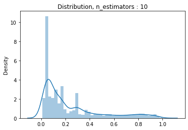
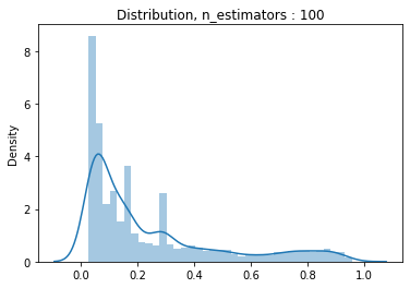
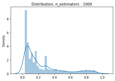
#n_estimator의 변화에 따른 분포분포

estimators = [1, 10, 100, 1000]

for estimator in estimators:

    pipe2 = make_pipeline(
    OrdinalEncoder(),
    SimpleImputer(),
    PolynomialFeatures(2),
    RandomForestClassifier(n_jobs = -1, random_state = 10, max_depth = 10,  max_features = 0.25, n_estimators = estimator)
    )

    pipe2.fit(X_train_val, y_train_val)

    y_pred_proba = pipe2.predict_proba(X_val)[:,1]

    dis = sns.distplot(y_pred_proba)
    dis.set_title('Distribution, n_estimators : {}'.format(estimator))
    plt.show()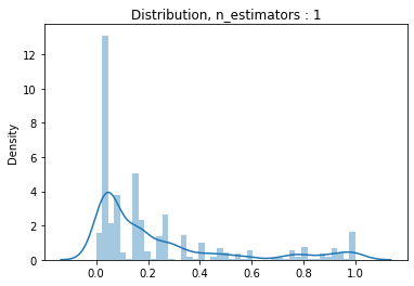
#ROC AUC를 통한 최종모델 결정 및 threshold 설정

from sklearn.metrics import roc_curve

pipe3 = make_pipeline(
    OrdinalEncoder(),
    SimpleImputer(),
    PolynomialFeatures(2),
    RandomForestClassifier(n_jobs = -1, random_state = 10, n_estimators = 200, max_depth = 10, max_features = 0.25, oob_score = True)
)

pipe3.fit(X_train_val, y_train_val)
y_pred_proba3 = pipe3.predict_proba(X_val)[:,1]

pipe4 = make_pipeline(
    OrdinalEncoder(),
    SimpleImputer(),
    PolynomialFeatures(2),
    RandomForestClassifier(n_jobs = -1, random_state = 10, n_estimators = 150, max_depth = 10, max_features = 0.25, oob_score = True)
)

pipe4.fit(X_train_val, y_train_val)
y_pred_proba4 = pipe4.predict_proba(X_val)[:,1]

pipe5 = make_pipeline(
    OrdinalEncoder(),
    SimpleImputer(),
    PolynomialFeatures(2),
    RandomForestClassifier(n_jobs = -1, random_state = 10, n_estimators = 100, max_depth = 10, max_features = 0.25, oob_score = True)
)

pipe5.fit(X_train_val, y_train_val)
y_pred_proba5 = pipe5.predict_proba(X_val)[:,1]
from sklearn.metrics import roc_auc_score
fpr3, tpr3, thresholds3 = roc_curve(y_val, y_pred_proba3)
plt.scatter(fpr3, tpr3)
plt.title('ROC curve')
plt.xlabel('FPR(Fall-out)')
plt.ylabel('TPR(Recall)');
# 최적의 threshold
optimal_idx = np.argmax(tpr3 - fpr3)
optimal_threshold = thresholds3[optimal_idx]
print('idx:', optimal_idx, ', threshold:', optimal_threshold)
print('AUC : ', roc_auc_score(y_val, y_pred_proba3))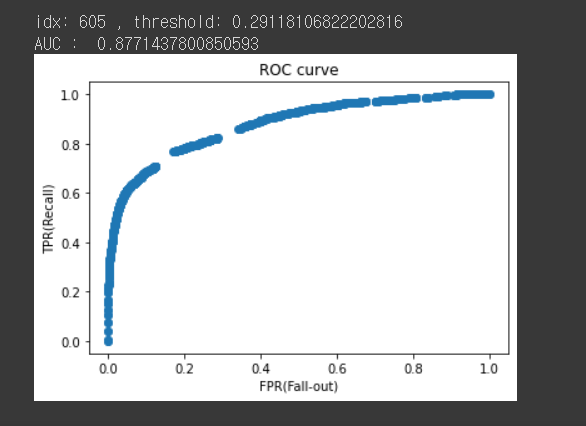
fpr4, tpr4, thresholds4 = roc_curve(y_val, y_pred_proba4)

plt.scatter(fpr4, tpr4)
plt.title('ROC curve')
plt.xlabel('FPR(Fall-out)')
plt.ylabel('TPR(Recall)');

# threshold 최대값의 인덱스, np.argmax()
optimal_idx = np.argmax(tpr4 - fpr4)
optimal_threshold = thresholds4[optimal_idx]

print('idx:', optimal_idx, ', threshold:', optimal_threshold)
print('AUC : ', roc_auc_score(y_val, y_pred_proba4))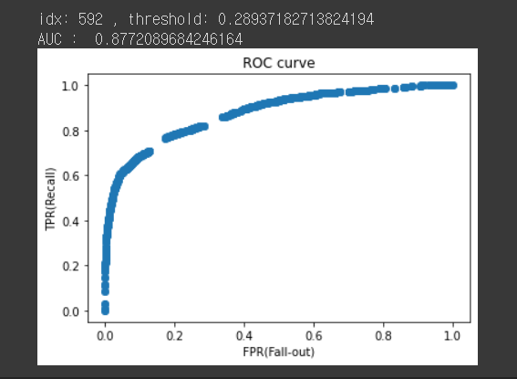
fpr5, tpr5, thresholds5 = roc_curve(y_val, y_pred_proba5)

plt.scatter(fpr5, tpr5)
plt.title('ROC curve')
plt.xlabel('FPR(Fall-out)')
plt.ylabel('TPR(Recall)');

# threshold 최대값의 인덱스, np.argmax()
optimal_idx = np.argmax(tpr5 - fpr5)
optimal_threshold = thresholds5[optimal_idx]

print('idx:', optimal_idx, ', threshold:', optimal_threshold)
print('AUC : ', roc_auc_score(y_val, y_pred_proba5))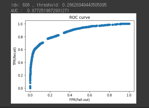
#kaggle submission 파일 생성kaggle submission 파일 생성

#test class 예측
y_pred_proba = pipe5.predict_proba(X_test)[:,1]
y_pred = y_pred_proba > 0.28626949443505095

#submission
result = pd.DataFrame(y_pred, columns = ['vacc_h1n1_f'])

result.reset_index(drop = False, inplace = True)

result.rename(columns = {
    'index' : 'id'
}, inplace = True)

result.set_index('id', inplace = True)

#submission 생성
result.to_csv('submission4_0416.csv')
회고
다양한 feature를 사용해보려고 노력하고 파라미터 튜닝을 진행했지만 원하는 만큼의 성과가 나오지는 못했다. 오히려 새로운 feature를 사용하지 않는 것이 더 높은 결과를 보여주는 경우도 있었다. 데이터에 대해 명확히 이해하지 못하고 무분별한 feature engineering은 독이될 수 있음을 깨달았다. 또한 데이터가 불균형인 데이터임에도 불구하고 별다른 조치없이 cross validation작업을 진행한 것도 좋은 결과가 나오지않은 이유 중 하나라고 생각된다. threshold를 어떻게 설정하느냐에 따라 모델성능이 꽤 크게 차이난다는 것도 알게되었다. 경험을 바탕으로 다음 캐글 대회에서는 더 발전해보자..
요약
1. 데이터 이해 중요
2. 불균형 데이터 cross validation시 stratify sampling 방법을 사용해주면 좋다.
3. threshold 잘 설정해야함
#불균형 데이터일때 사용하면 좋은 cross validation 함수

from sklearn.mode_selection import StratifiedkFold

StratifiedKFold(n_splits=5, *, shuffle=False, random_state=None)[source]