사이킥런에서 제공하는 붓꽃(Iris) 데이터를 활용해 품종을 분류(Classification)을 실행
분류(Classification) : 독립변수값이 주어졌을 때 그 값과 가장 연관성이 큰 종속변수값
(클래스)을 예측하는 문제
데이터 유형 : 150x4 numpy.ndarray
↳ feature : 꽃받침 길이, 꽃받침 너비, 꽃잎 길이, 꽃잎 너비
↳ 정답 label : 3가지(Setosa, Versicolour, Virginica)
↳ data.target에는 setosa : 0, versicolour : 1, virginica : 3 으로 매핑되어있음
목표 : 150개의 붓꽃 데이터 중 70%를 train set, 30%를 test set으로 나눈 후 만들어진 모델의 accuracy 출력.
데이터 전처리 및 시각화를 위한 패키지와 iris 데이터를 import한다
import pandas as pd
import numpy as np
import matplotlib.pyplot as plt
import seaborn as sns
from sklearn.datasets import load_iris
iris 데이터의 기본 shape를 확인
#dataset load
data = load_iris()

#separating dataset
features = data.data    # (150, 4)의 예측변수값
feature_names = data.feature_names #피쳐 이름
target = data.target #정답 컬럼값
target_names = data.target_names #정답 컬럼 이름

print(features.shape, target.shape)

(150, 4) (150,)
특징의 이름과, 타겟의 이름도 확인한다
feature_names

['sepal length (cm)',
 'sepal width (cm)',
 'petal length (cm)',
 'petal width (cm)']

target_names

array(['setosa', 'versicolor', 'virginica'], dtype='<U10')
전처리를 하기 위해선 DataFrame 형태가 더 편하기 때문에 변환
all_data = pd.DataFrame(features, columns=feature_names)
all_data['target'] = target
all_data.info()

class 'pandas.core.frame.DataFrame'>
RangeIndex: 150 entries, 0 to 149
Data columns (total 5 columns):
 #   Column             Non-Null Count  Dtype
---  ------             --------------  -----
 0   sepal length (cm)  150 non-null    float64
 1   sepal width (cm)   150 non-null    float64
 2   petal length (cm)  150 non-null    float64
 3   petal width (cm)   150 non-null    float64
 4   target             150 non-null    int64
dtypes: float64(4), int64(1)
memory usage: 6.0 KB
데이터 자체가 결측치가 없고, 수가 많지 않기 때문에 시각화를 하여 쉽게 데이터 사이의 관계를 확인할 수 있다
sns.pairplot(all_data, hue='target', size=3)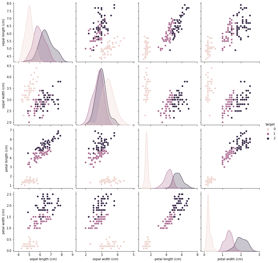
데이터 간의 상관계수를 수치로 표현하기 위해 corr() 함수를 이용한다
corr = all_data
corr = corr.corr(method='pearson')
corr['target'].drop(['target'])

sepal length (cm)    0.782561
sepal width (cm)    -0.426658
petal length (cm)    0.949035
petal width (cm)     0.956547
Name: target, dtype: float64
절대값 0.3 이상이기 때문에 전부 사용한다
sns.heatmap(corr, annot=True, cmap='RdYlBu_r', vmin=-1, vmax=1)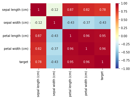
히트맵 출력
plt.figure(figsize = (12,6))
sns.boxplot(x='petal length (cm)', y='target', data=all_data, orient='h')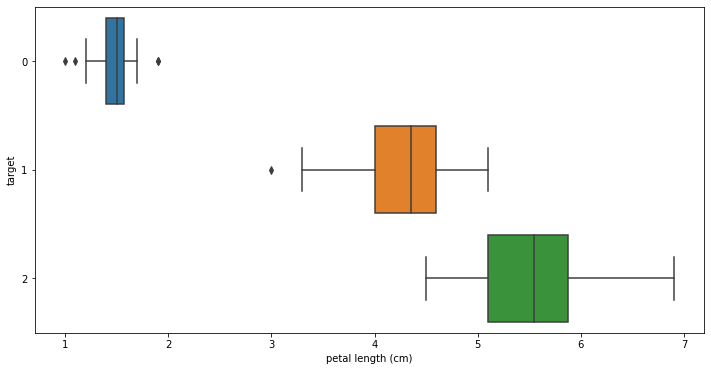
plt.figure(figsize = (12,6))
sns.boxplot(x='petal width (cm)', y='target', data=all_data, orient='h')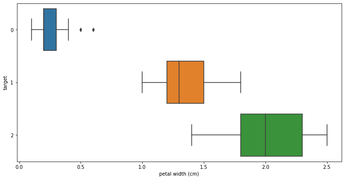
상관계수가 높은 petal length와 petal width를 boxplot로 출력해준다
이상치가 출력되는 것을 확인할 수 있다
이상치를 해결하기 위해 어떤 스케일러를 사용할 지 고민할 필요가 있다
from sklearn.model_selection import train_test_split

x_train, x_test, y_train, y_test = train_test_split(all_data.iloc[:,:-1], all_data.iloc[:,-1:], test_size=0.3)

print(x_train.shape, x_test.shape, y_train.shape, y_test.shape)
이제 학습을 위해 데이터를 학습 데이터와 테스트 데이터로 나눠준다
함수는 사이킥런에서 제공하는 train_test_split를 사용했으며, 7:3 비율로 나눠줬다
from sklearn.pipeline import make_pipeline # 한 번에 처리하는 파이프라인 생성
from sklearn.linear_model import LogisticRegression # 로지스틱 회귀
from sklearn.svm import SVC # 서포트벡터머신
from sklearn.ensemble import RandomForestClassifier # 랜덤포레스트
from sklearn.neighbors import KNeighborsClassifier # k-최근접이웃
from sklearn.metrics import accuracy_score # 정확도 측정
import warnings
warnings.filterwarnings(action='ignore') # 경고창 무시
그 후 학습을 위한 모듈들을 import한다
lr = LogisticRegression()
svc = SVC(C=1.0, kernel='linear')
rfc = RandomForestClassifier(n_estimators=100)
knn = KNeighborsClassifier(n_neighbors = 3)
그 후 모델들을 생성한다
scv : C는 오류 허용도로 작을수록 많은 오류를 허용한다, C값을 여러번 넣으며 확인해야 하는데, overfitting되는 경우 작은 값을 지정하여 규제할 수 있다. kernel은 linear을 지정하여 선형으로 결정경계를 정한다
rfc : 랜덤포레스트는 여러개의 결정트리로 구성되어 있으며 n_estimators은 분류기의 개수를 정해준다
knn : k-최근접 이웃은 특정 점으로부터 계수 만큼 주변 target을 파악해 분류를 수행하는 모델이다. 여기선 3을 지정해 점에서 가장 가까운 3개의 target를 파악해 분류를 수행한다
models = [lr, svc, rfc, knn]

for model in models:
  model.fit(x_train, y_train)
  y_pred = model.predict(x_test)

  accuracy = accuracy_score(y_test, y_pred)
  print(f"modle : {model}\n accuracy : {accuracy}\n")
그 후 for문을 이용해 모델명과 성능을 출력한다
modle : LogisticRegression()
 accuracy : 0.9777777777777777

modle : SVC(kernel='linear')
 accuracy : 1.0

modle : RandomForestClassifier()
 accuracy : 0.9555555555555556

modle : KNeighborsClassifier(n_neighbors=3)
 accuracy : 0.9555555555555556
svc 모델이 가장 좋은 성능을 보인다
Scaler와 PCA
사이킥런은 데이터 전처리에 필요한 다양한 스케일러를 제공한다
-
StandardScaler : 표준화, 평균을 제거하고 데이터를 단위 분산으로 조정
-
MinMaxScaler : 정규화, 모든 feature 값이 0~1사이에 있도록 데이터를 재조정
-
RobustScaler : 이상치 영향 최소화, 중간값과 IQR(25%~75% 범위의 데이터를 스케일링)을 사용
여기서 주의할 점은 학습 데이터에 대해서만 fit()을 적용해야 한다는 것이다
테스트 데이터로 다시 fit을 적용하면 기준이 다시 달라지기 때문에 올바른 학습을 수행할 수 없다
차원의 저주 : 수학적 공간 차원이 늘어나면 문제의 계산법이 지수적으로 커지는 문제
데이터가 차원은 높은데 개수가 적기 때문에 과대적합한 모델이 완성된다
원활한 학습을 위해선 차원을 축소시키거나, 데이터를 많이 수집해야 한다
PCA : 차원을 축소하는 방법으로 특징추출에 해당된다
데이터의 분산을 최대한 보존하면서 서로 직교하는 주성분을 찾아, 고차원 공간의 표본들을 저차원 공간으로 변환하는 기법으로, 특이값분해(SVD)를 사용한다
iris 데이터를 활용해 pca를 적용한다
이때 n_components는 유지할 주성분의 수 혹은 비율로, 2를 지정하여 주성분을 2개 남긴다
from sklearn.preprocessing import StandardScaler
from sklearn.decomposition import PCA

x = StandardScaler().fit_transform(data.data)
y = data.target

pca = PCA(n_components=2)
pca_x = pca.fit_transform(x)
df = pd.DataFrame(pca_x, columns=['f1', 'f2'])
df

	f1	f2
0	-2.264703	0.480027
1	-2.080961	-0.674134
2	-2.364229	-0.341908
3	-2.299384	-0.597395
4	-2.389842	0.646835
...	...	...
145	1.870503	0.386966
146	1.564580	-0.896687
147	1.521170	0.269069
148	1.372788	1.011254
149	0.960656	-0.024332
150 rows × 2 columnsplt.plot(pca_x[:,0][y==0], pca_x[:,1][y==0], "ro", markersize=3, label='setosa')
plt.plot(pca_x[:,0][y==1], pca_x[:,1][y==1], "g^", markersize=3, label='versicolor')
plt.plot(pca_x[:,0][y==2], pca_x[:,1][y==2], "bs", markersize=3, label='virginica')
plt.xlabel('feature 1')
plt.ylabel('feature 2')
plt.legend()
plt.show()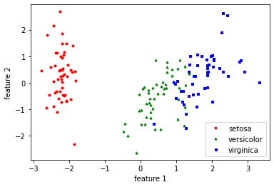
결과를 시각화하여 확인한다
lr = make_pipeline(StandardScaler(), PCA(), LogisticRegression())
svc = make_pipeline(StandardScaler(), PCA(), SVC(C=1.0, kernel='linear'))
rfc = make_pipeline(StandardScaler(), PCA(), RandomForestClassifier(n_estimators=10))
파이프라인을 이용해 Standardscaler와 PCA기법을 적용시킨 후 학습을 진행한다
models = [lr, svc, rfc]

for model in models:
  model.fit(x_train, y_train)
  y_pred = model.predict(x_test)

  accuracy = accuracy_score(y_test, y_pred)
  print(f"modle : {model}\n accuracy : {accuracy}\n")
modle : Pipeline(steps=[('standardscaler', StandardScaler()), ('pca', PCA()),
('logisticregression', LogisticRegression())])
accuracy : 0.9555555555555556
modle : Pipeline(steps=[('standardscaler', StandardScaler()), ('pca', PCA()),
('svc', SVC(kernel='linear'))])
accuracy : 0.9777777777777777
modle : Pipeline(steps=[('standardscaler', StandardScaler()), ('pca', PCA()),
('randomforestclassifier',
RandomForestClassifier(n_estimators=10))])
accuracy : 0.9555555555555556오히려 학습률이 떨어졌다
그렇게 때문에 상황에 맞는 적절한 스케일러와 특징추출을 진행해야 좋은 성능을 가진 모델을 생성할 수 있다