Day7 - R(7). 22.08.31.수

[어제 복습]

1. "~.txt" 읽는방법
   :read_lines(),read.csv() /
   read.csv('.txt', fileEncoding = 'cp949')
   readLines('.txt')

2.???
1차원:백터
2차원:데이터프레임(숫자, 문자) 데이터프레임안에 데이터플레임 못들어감.
3차원:리스트
:unlist

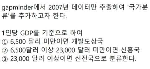
:gapminder <- gapminder %>% filter(year== 2007)
gapminder$'국가분류' <- ifelse(gapminder$gdpPercap < 6500, '개발도상국', ifelse(gapminder$gdpPercap < 23000, '신흥국', '선진국'))

:gdf %>% group_by(국가분류) %>%
summarise(기대수명평균 = mean(lifeExp)) %>%
ggplot(aes(x=국가분류, y=기대수명평균, fill=국가분류)) + geom_col() + coord_filp()

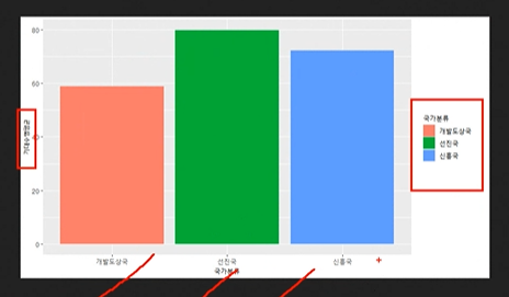
: + scale_x_discrete(limits = c(""))

:mpg1 <- mpg %>% filter(model == "toyota tacoma 4wd" )
range(mpg1$displ) :mpg$displ)

7. mpg $ manufacturer를 wordcloud()로 표현해라
   :df <- as.data.frame(table(mpg$manufacturer))
   wordcloud2(df)

   ---

   [8/31일 R수업]

• 감성분석기법: 상품 및 서비스, 기관이나 단체, 사회적 이슈, 사건 등에 관 하여 블로그 또는 트위터, 페이스북과 같은 소셜 미디 어 등에 남긴 의견을 수집하고 분석하여 사람들의 감정 의 상태 및 태도에 대한 변화, 의견과 평가, 선호 등을 파악하는 빅데이터 분석 기술을 말한다

설치하기

(파일 주심)

• package1 <- c("ggplot2", "Rcpp", "dplyr", "ggthemes", "ggmap", "devtools", "RCurl", "igraph", "rgl", "lavaan", "semPlot")
• package2 <- c("twitteR", "XML", "plyr", "doBy", "RJSONIO", "tm", "RWeka", "base64enc")
• list.of.packages <- c( package1, package2)
  new.packages <- list.of.packages[!(list.of.packages %in% installed.packages()[,"Package"])]
• if(length(new.packages)) install.packages(new.packages)
• library(plyr)
• library(stringr)

삼성

• load("samsung_tweets.rda")
• samsung_tweets
• library(twitteR)
• st <- twListToDF(samsung_tweets)
• head(st,2)
• names(st)

• st_text <- st$text
• st_text

필요없는 내용 지우기 - 알바벳과 숫자를 제외한 나머지 모든것을 찾아서 지워라 = W의미

• 👌st_text <- gsub("\\W"," ", st_text) #치환할때 자주 사용함

• st_text

• st_df <- as.data.frame(st_text)

• st_df

애플

• load("apple_tweets.rda")

• library(twitteR)

• at <- twListToDF(apple_tweets)

• head(at,2)

• names(at)

• at_text <- at$text

• at_text

• at_text <- gsub("\W"," ", at_text)

• at_text

• at_df <- as.data.frame(at_text)

• at_text

• at_df <- as.data.frame(at_text)

---

#감성사전 https://github.com/The-ECG/BigData1_1.3.3_Text-Mining ===========

(파일주심)
pos.word <- scan("positive-words.txt", what ="character", comment.char = ";")
neg.word <- scan("negative-words.txt", what ="character", comment.char = ";")

#https://stackoverflow.com/questions/35222946/score-sentiment-function-in-r-return-always-0

score.sentiment = function(sentences, pos.words, neg.words, .progress='none')
{
scores = laply(sentences, function(sentence, pos.words, neg.words) {
sentence = gsub('[^A-z ]','', sentence)
sentence = tolower(sentence);
word.list = str_split(sentence, '\s+');
words = unlist(word.list);
pos.matches = match(words, pos.words);
neg.matches = match(words, neg.words);
pos.matches = !is.na(pos.matches);
neg.matches = !is.na(neg.matches);
score = sum(pos.matches) - sum(neg.matches);
return(score);
}, pos.words, neg.words, .progress=.progress);
scores.df = data.frame(score=scores, text=sentences);
return(scores.df);
}

---

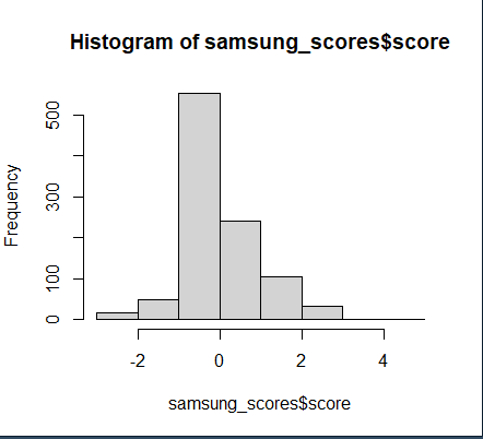
삼성 스코어

• samsung_scores <- score.sentiment(st_text, pos.word , neg.word, .progress = 'text')

• head(samsung_scores,2)

• samsung_scores$score

• hist(samsung_scores$score)

---

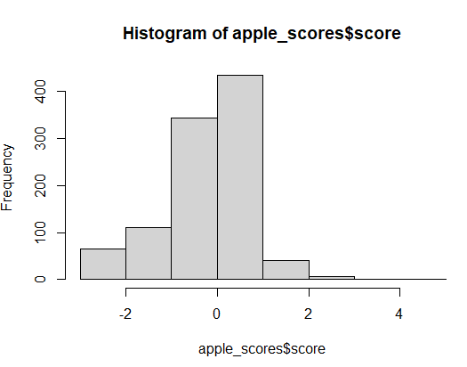
애플 스코어

• apple_scores <- score.sentiment(at_text, pos.word , neg.word, .progress = 'text')

• head(apple_scores,2)

• apple_scores$score

• hist(apple_scores$score)

---

• 행의 갯수를 변수로 정해줌

• a <- dim(samsung_scores)[1]
• b <- dim(apple_scores)[1]

• 데이터 수 확인:
  length : 길이반환 , dim : 차원반환, nrow : 행의 수 반환, ncol : 열의수 반환

• alls <- rbind(as.data.frame(cbind(type=rep("samsung",a),score=samsung_scores[,1])),
  as.data.frame(cbind(type=rep("apple",b),score=apple_scores[,1])))

• R 데이터 프레임의 결합: rbind() : 행결합, cbind() : 열결합, merge()

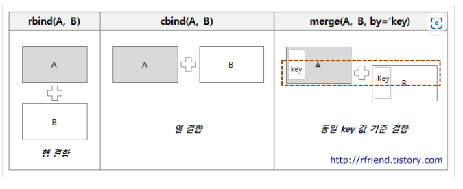
• rep(a,b):a를 b만큼 반복하겠다.

# 백터형으로 바꾼 이유는? -> :
#type->백터 변환,core->정수형 변환

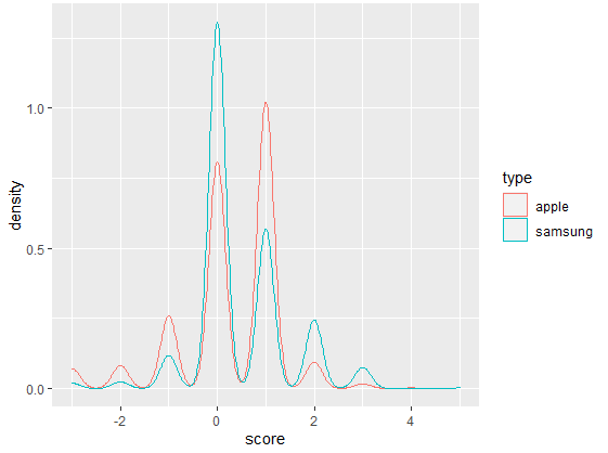
• alls $ type <- factor(alls$type)

• alls $ score <- as.integer(alls$score)

• ggplot(alls,aes(x=score,colour=type))+geom_density()

---

[오후 수업]

• 단순 선형 회귀분석

단순선형회귀분석 -> 독립변수 1개 라는 의미
linear, 선형

직선을 찾아주는것
회귀: 기준으로 돌아간다
:x-> 설명변수, y-> 반응변수
회귀는 인과관계를 가정한다.
회귀개수 x,y
잘 설명하고있다=오차가 적었다.
오차제곱 합의 평균 루트 r 평균m 제곱s 오e
잔차제곱
[비용함수 cost]를 최소로 낮추는 것.
그때의 x, y값을 찾아내자
r2의 값은 클수록 좋다.
lm(y~x,data=):y는 x를 따른다. 정규분포.
lnear model

plot(),paris()

상관계수 :소문자r
상관행렬:cor()

---

str(cars)

ggplot(cars,aes(x=speed,y=dist))+geom_point()

r2
cor.test(cars$speed,cars$dist)
install.packages("corrplot")
library(corrplot)

fit.cars <- lm(dist ~ speed, data=cars)
fit.cars
summary(fit.cars)
str(fit.cars)
names(fit.cars)

#predict('lm'으로 만들어진결과물,newdata, *,se.fit=FALSE, scale=NULL, df=Inf):예측하다

predict(fit.cars,data.frame( speed=20))

data.frame( speed=20)

predict(fit.cars,data.frame( speed=20),interval = "confidence")
predict(fit.cars,data.frame( speed=c(20,120)),interval = "confidence")

ggplot(data=mpg,aes(x=displ, y=cty,color=drv))+geom_point()+geom_smooth(method = 'lm')

---

출처:
https://rfriend.tistory.com/51 <- R 데이터 프레임 결합
https://rbasall.tistory.com/79 <- 데이터 수 확인