01_What is Machine Learning - 머신러닝이란
머신이 배운다~
데이터로부터 머신이 배운다
명시적인 프로그램에 의해서가 아니라, 주어진 데이터를 통해 규칙을 찾는것
원리는 뭘까?
02_What is Machine Learning - 데이터관찰(휴먼러닝)
iris classification
아이리스 품종을 맞출 수 있을까?
iris=load_iris()iris.keys()dict_keys(['data', 'target', 'frame', 'target_names', 'DESCR', 'feature_names', 'filename', 'data_module'])
print(iris['DESCR']).. _iris_dataset:
Iris plants dataset
Data Set Characteristics:
:Number of Instances: 150 (50 in each of three classes)
:Number of Attributes: 4 numeric, predictive attributes and the class
:Attribute Information:
    - sepal length in cm
    - sepal width in cm
    - petal length in cm
    - petal width in cm
    - class:
            - Iris-Setosa
            - Iris-Versicolour
            - Iris-Virginica

:Summary Statistics:

============== ==== ==== ======= ===== ====================
                Min  Max   Mean    SD   Class Correlation
============== ==== ==== ======= ===== ====================
sepal length:   4.3  7.9   5.84   0.83    0.7826
sepal width:    2.0  4.4   3.05   0.43   -0.4194
petal length:   1.0  6.9   3.76   1.76    0.9490  (high!)
petal width:    0.1  2.5   1.20   0.76    0.9565  (high!)
============== ==== ==== ======= ===== ====================

:Missing Attribute Values: None
:Class Distribution: 33.3% for each of 3 classes.
:Creator: R.A. Fisher
:Donor: Michael Marshall (MARSHALL%PLU@io.arc.nasa.gov)
:Date: July, 1988
The famous Iris database, first used by Sir R.A. Fisher. The dataset is taken
from Fisher's paper. Note that it's the same as in R, but not as in the UCI
Machine Learning Repository, which has two wrong data points.
This is perhaps the best known database to be found in the
pattern recognition literature. Fisher's paper is a classic in the field and
is referenced frequently to this day. (See Duda & Hart, for example.) The
data set contains 3 classes of 50 instances each, where each class refers to a
type of iris plant. One class is linearly separable from the other 2; the
latter are NOT linearly separable from each other.
.. topic:: References
- Fisher, R.A. "The use of multiple measurements in taxonomic problems"
Annual Eugenics, 7, Part II, 179-188 (1936); also in "Contributions to
Mathematical Statistics" (John Wiley, NY, 1950). - Duda, R.O., & Hart, P.E. (1973) Pattern Classification and Scene Analysis.
(Q327.D83) John Wiley & Sons. ISBN 0-471-22361-1. See page 218. - Dasarathy, B.V. (1980) "Nosing Around the Neighborhood: A New System
Structure and Classification Rule for Recognition in Partially Exposed
Environments". IEEE Transactions on Pattern Analysis and Machine
Intelligence, Vol. PAMI-2, No. 1, 67-71. - Gates, G.W. (1972) "The Reduced Nearest Neighbor Rule". IEEE Transactions
on Information Theory, May 1972, 431-433. - See also: 1988 MLC Proceedings, 54-64. Cheeseman et al"s AUTOCLASS II
conceptual clustering system finds 3 classes in the data. - Many, many more ...
iris_pd = pd.DataFrame(iris.data, columns=iris.feature_names)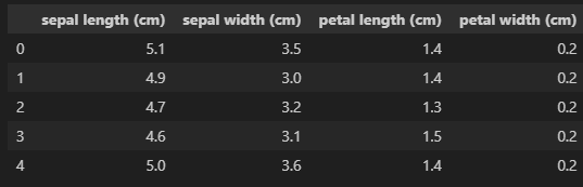
이런 상황에서 어떻게 맞출 수 있을까?
- 기존 3종에 대해 먼저 공부하고 (sepal, petal & width, length에 대해 파악)
- 아이리스 꽃 품종을 맞출수 있나 확인해보면됨
일단 관계를 확인해보자
plt.figure(figsize=(12,6))
sns.boxplot(x='sepal length (cm)', y='species', data= iris_pd, orient='h')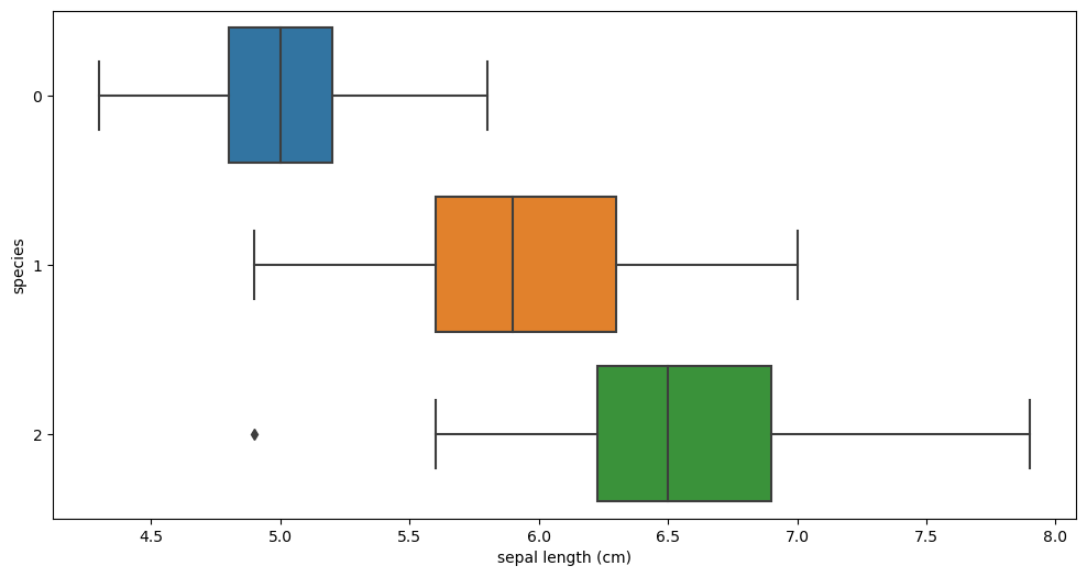
plt.figure(figsize=(12,6))
sns.boxplot(x='sepal width (cm)', y='species', data= iris_pd, orient='h')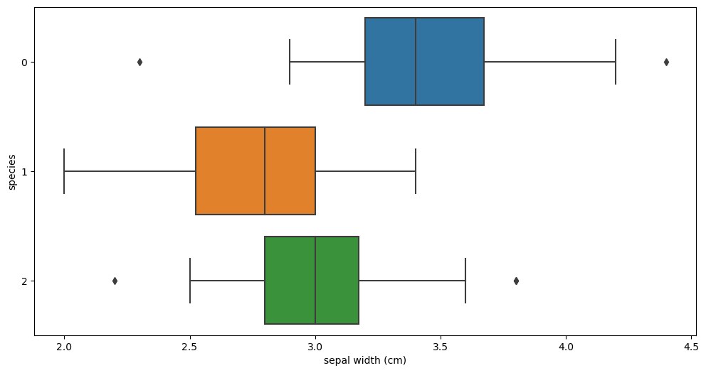
plt.figure(figsize=(12,6))
sns.boxplot(x='petal length (cm)', y='species', data= iris_pd, orient='h')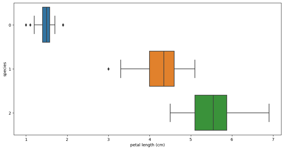
plt.figure(figsize=(12,6))
sns.boxplot(x='petal width (cm)', y='species', data= iris_pd, orient='h')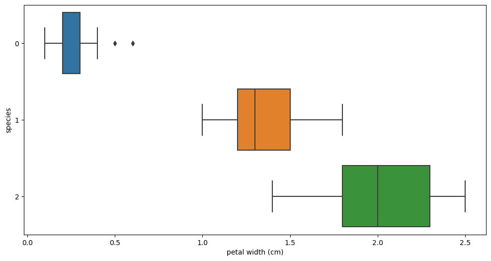
petal length, width가 오히려 구분이 더 잘된다(겹치는 구간이 적다!
그래도 아직까지는 꼬리쪽이 겹쳐보임에 따라 명확한 구분은 어려워보임
추가 확인
sns.pairplot(iris_pd, hue='species')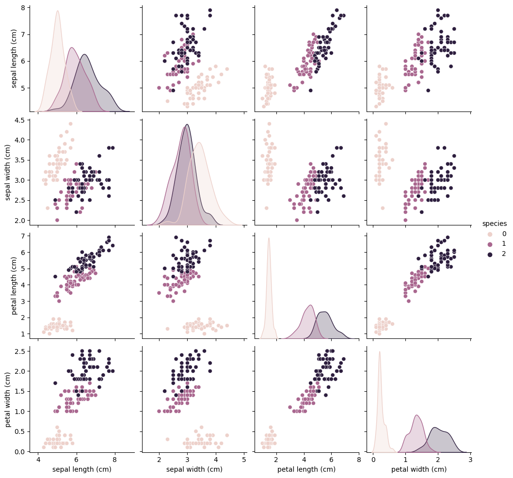
음! 이렇게 봐도 petal length, width로 구분하는게 가장 적합해보임
speices중 0번은 그냥 더디가 다져다 놔도 잘 구분되어보임
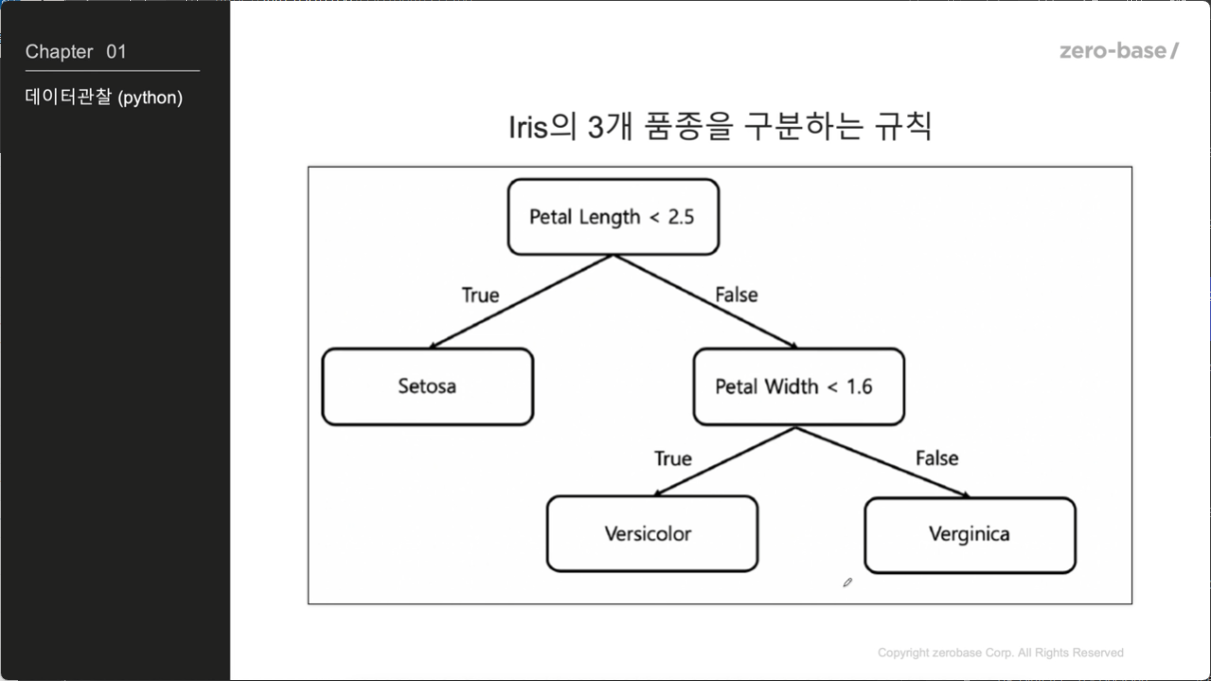
품종 세개를 구분할 수 있을까?
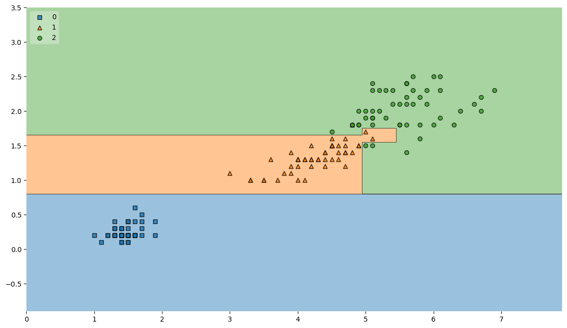
sns.relplot(data=iris_pd, x='petal length (cm)', y='petal width (cm)', hue = 'species')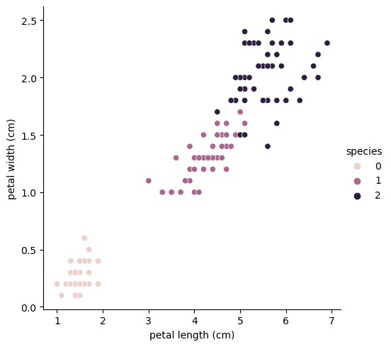

몇개의 데이터는 놓치겠지만, petal width가 1.65정도에 잘라서
versicolor(주황, 1)는
- petal length 가 2.9보다 크면서, petal width가 1.6보다 작은 경우
virginica(빨강, 2)는
- petal length 가 5보다 크면서, petal width가 1.75보다 큰 경우
이런 내용을 질문(조건문)으로 순차적으로 표현한 것이 decision tree
이게 최선일까..?
이럴때 알고리즘 등장
현재 상황에서 이것이 최선이라는 근고
혹은 이런방향, 저런 방향으로 진행했을 때 각각의 차이점에 대한 정량적 수치 제시
내가 임의로 정한 저 가로 세로 선이 어디에 있는 것이 최선일지 확인해야함
03 What is Machine Learning - Decision Tree
상황 설정
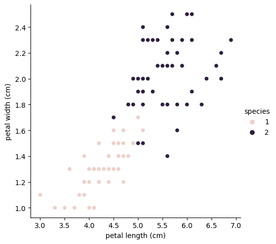
species 0번, setosa구분은 너무 잘되니 1,2번 구분짓는 선을 어떻게 잘 찾을 것인가
iris_12=iris_pd[iris_pd['species']!=0]

sns.relplot(data=iris_12, x='petal length (cm)', y='petal width (cm)', hue = 'species')
species 1, 2만 빼내기
decision tree를 위한 정보획득(information gain)
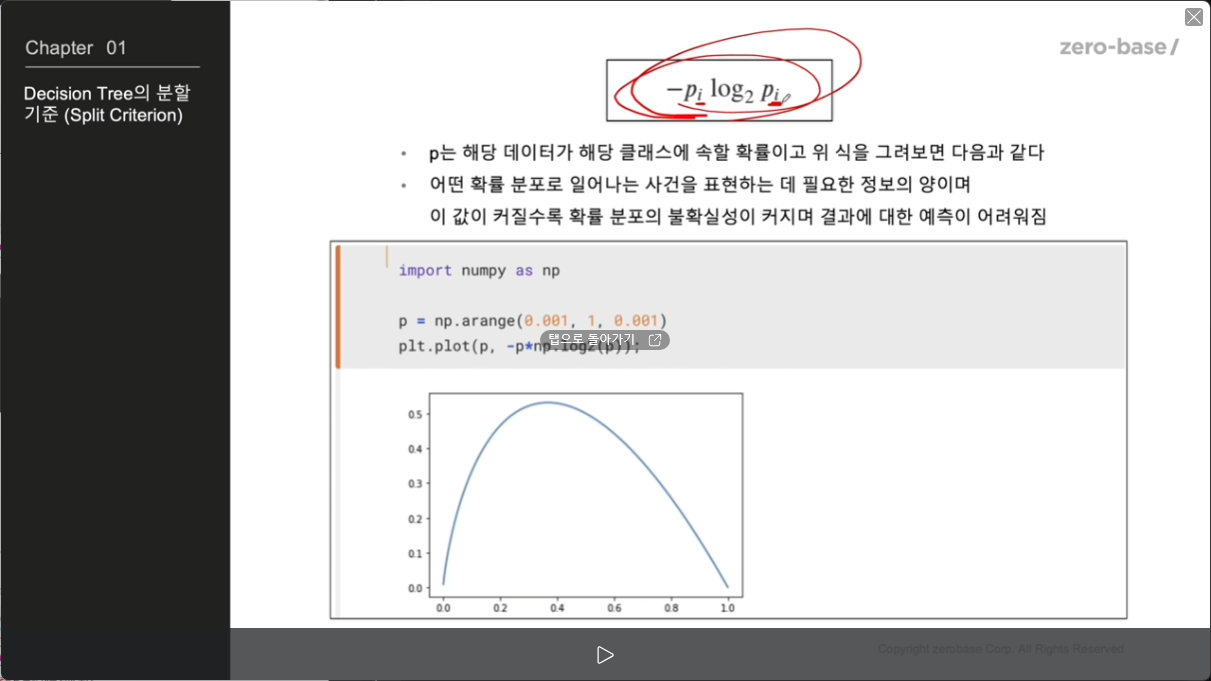
정보의 가치를 반환하는데 발생하는 사전의 확률이 작을수록 정보의 가치는 커진다.
정보 이득이란 어떤 속성을 선택함으로 인해서 데이터를 더 잘 구분하게 되는 것
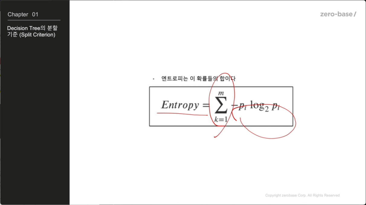
엔트로피 개념
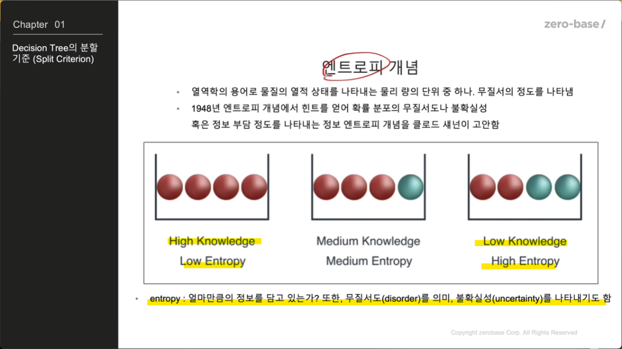
<공을 뽑는 것에 대한 엔트로피>
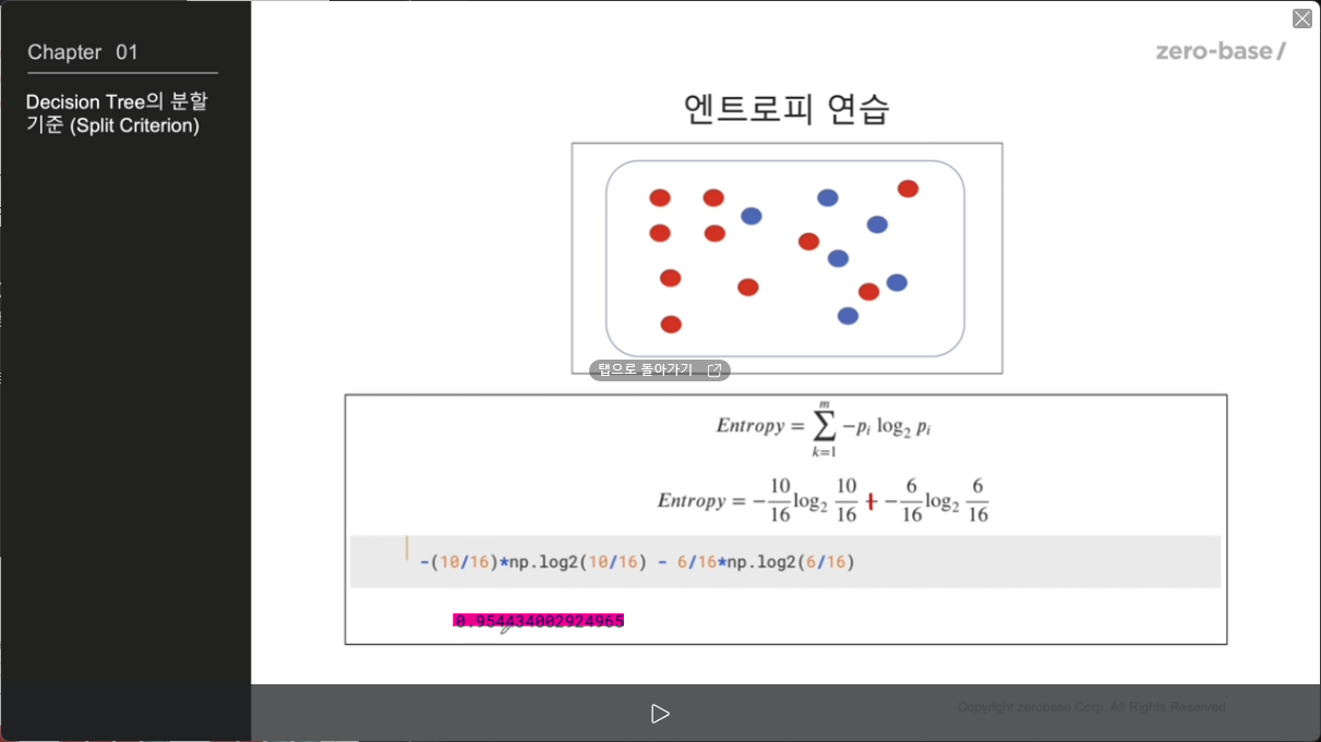
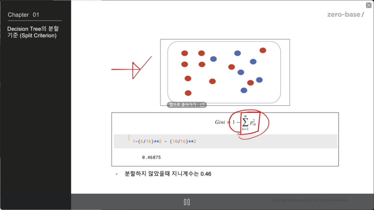
안나눴을때 엔트로피 : 0.9~
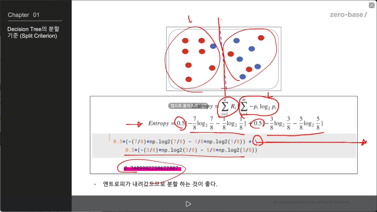
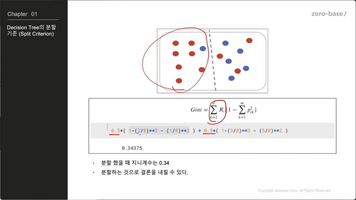
나누고 나서 엔트로피 : 0.7
나누고 나서 엔트로피가 더 낮으니 나눠야함.
그런데,
log는 컴퓨터 계산하는 속도에 영향을 미침.
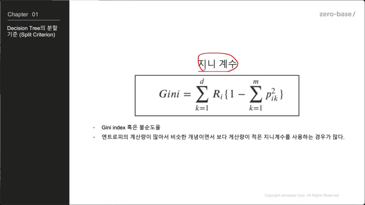
따라서 그를 보완한 것이
지니계수
따라서
species를 세분화하여 나눠보고 가장 적합한 엔트로피를 가진 포인트를 잡으면 됨
04 What is Machine Learning - scikit learn
decision tree를 직접 코딩하지 않아도 된다..
휴
from sklearn.tree import DecisionTreeClassifier
from sklearn.metrics import accuracy_score

iris_tree = DecisionTreeClassifier()
iris_tree.fit(iris.data[:,2:]# 모든 행에2,3번만 가져와서 봐라, 1번은 안봐도 구분 가능
, iris.target# 정답은 이거야 라고 알려주기
) #공부해줘, 여기 데이터 줄거고 이거를 통해 추후에 도출되어야하는 데이터는 이거인데 이게 데이터에 대한 정답이다~
y_pred_tr = iris_tree.predict(iris.data[:,2:]) #공부를 마친 iris_tree한테, iris.data[:,2:]를 주고 맞춰봐라 하는거y_pred_tr
iris.target #실제답은?
accuracy_score(iris.target, y_pred_tr) #정답은 iris.target, 너가 말해준 답은 y_pred_tr 정답률 봐라0.9933333333333333
05 데이터나누기 - Decision Tree를 이용한 Iris 분류 - 과적합
이 전까지 했던 것은 지도학습임
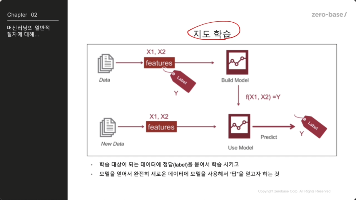
정답을 알려주고 학습을 시킨뒤
새로운 데이터를 준다음 학습한 내용을 이용해서 결과를 예측해보기
그러면 그 지도학습으로 어떻게 tree가 그려졌나 확인해보면
from sklearn.tree import plot_tree
plt.figure(figsize=(12,8))
plot_tree(iris_tree)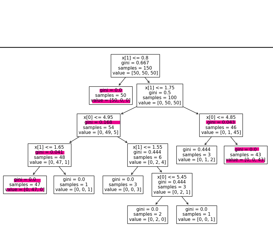
그러면 저 지니계수를 가지고 나눠놓은 것을 함 확인해보자
저 복잡한 트리의 결과가 이거임
저 결과로 99%정확도가 나온건데...
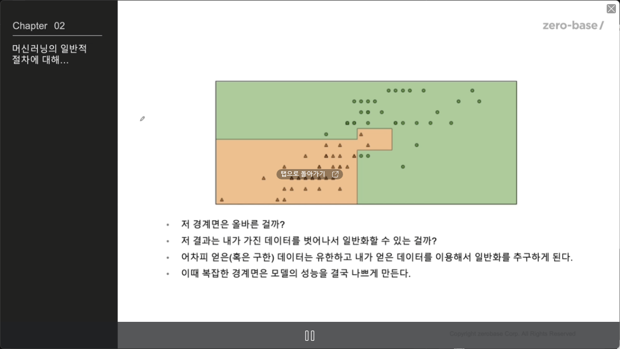
- 예외값이 저 데이터 한정 예외값일거 아닐까?
너무 딱맞게 99%정확도 맞게 나오는게 맞는걸까?
과적합 : 내가 가진 데이터에만 너무 fix 한 상태. 다른 데이터에는 정확도 낮은 상태
06 데이터나누기 - Decision Tree를 이용한 Iris 분류 - 데이터나누기
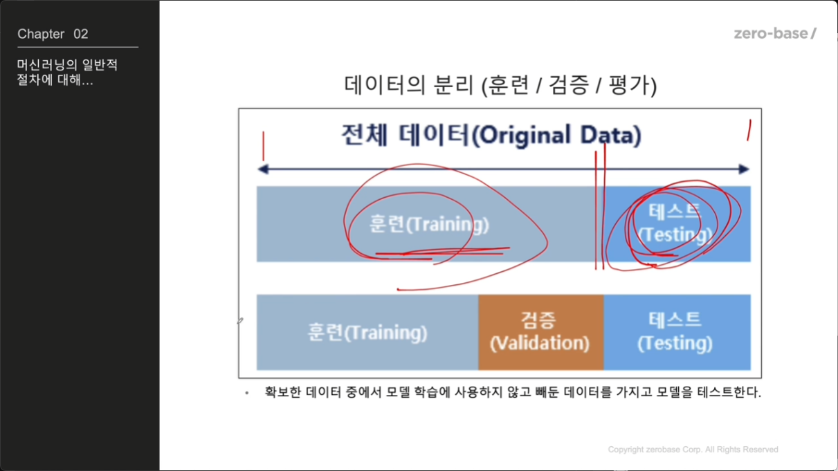
데이터는 나눠야한다. 과적합을 피하기 위해
데이터의 일부는 훈련으로 쓰고
또 일부는 훈련에 대한 검증으로 쓰고
마지막 일부는 테스트 용으로 써야한다
모든것을 훈련 및 테스트 용으로 쓰면 과적합난다
데이터를 훈련/테스트로 분리
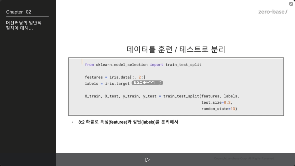
from sklearn.model_selection import train_test_split

features = iris.data[:, 2:]
labels = iris.target

features = iris.data[:, 2:]
labels = iris.target

x_train, x_test, y_train, y_test = train_test_split(features, labels,
				test_size = 0.2,
                stratify=labels,# 분포 맞춰주기
                random_state=13)
이제 train 데이터로 decision tree 만들어보기
iris_tree = DecisionTreeClassifier(max_depth=2, #트리에서 2단계까지만 내려가라고 지정, 그런데 깊이 내려갈수록 내 데이터에 완전 fit 해짐, 그런데 내 데이터에 fit 해지면 과적합난다. 따라서 규제.
                                   random_state=13)
iris_tree.fit(x_train,y_train)

plot_tree(iris_tree)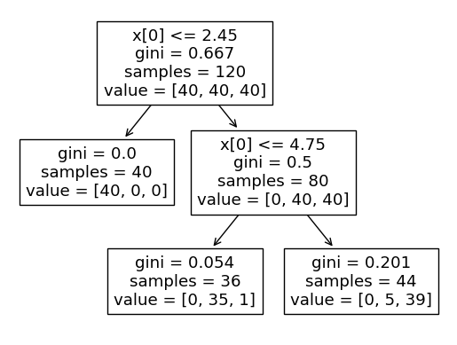
그러면 트리 결과 확인해보기
y_pred_tr = iris_tree.predict(iris.data[:,2:])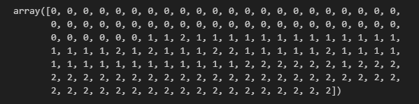
accuracy_score(iris.target, y_pred_tr) 0.9533333333333334
아까보다는 낮아졌다!
그러면 이 트리로 어떻게 나눠놨는지 함 보자 (결정경계)
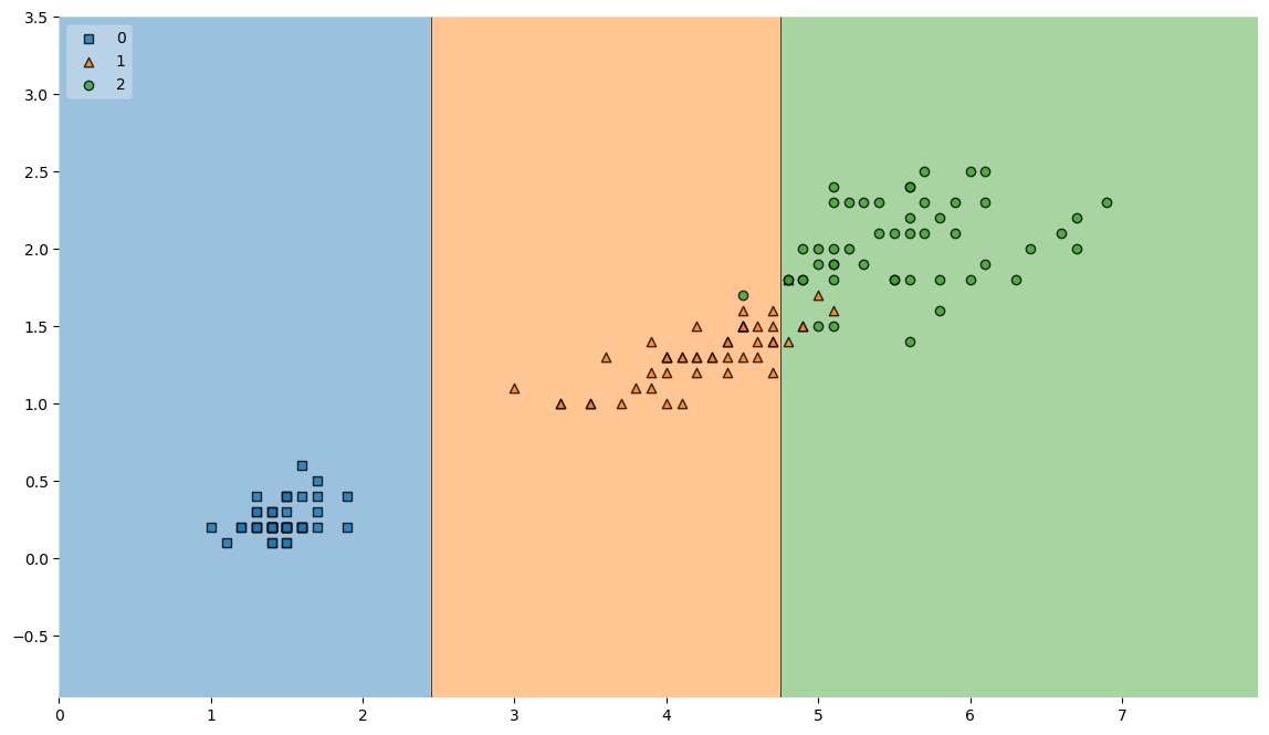
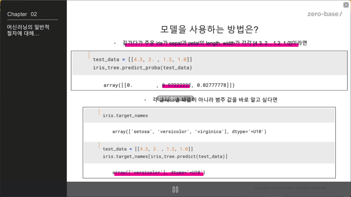
자 이제, 모델을 사용하는 방법은?
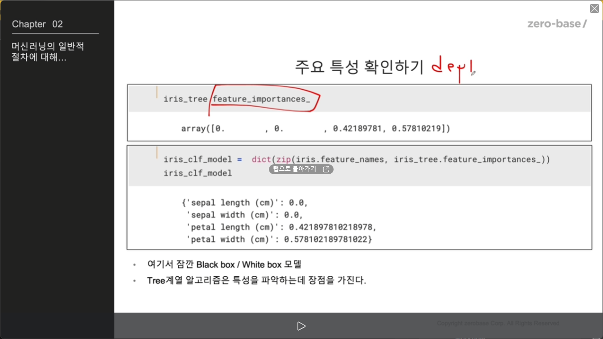
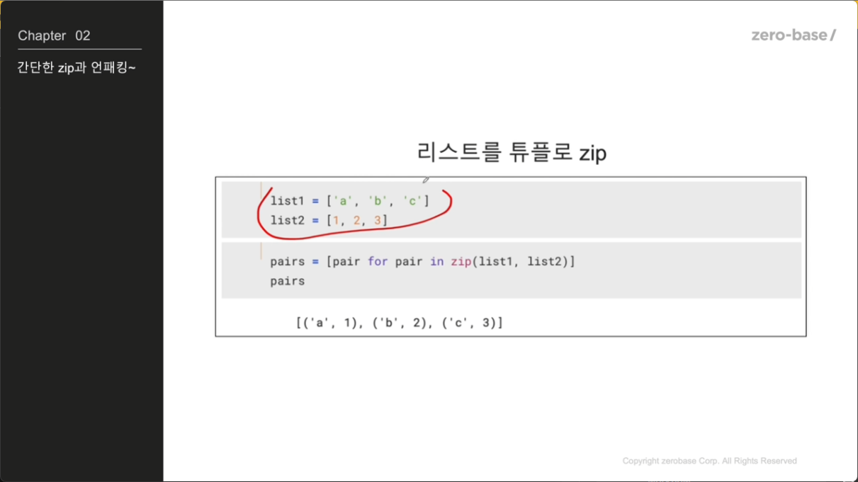
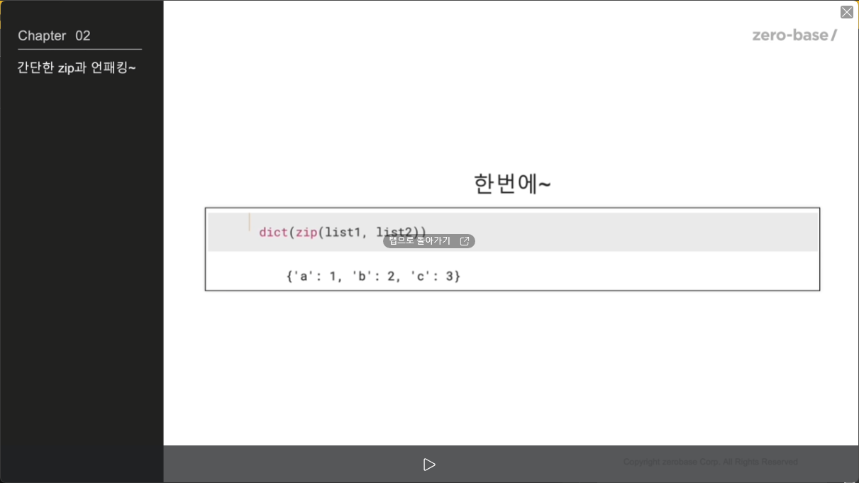
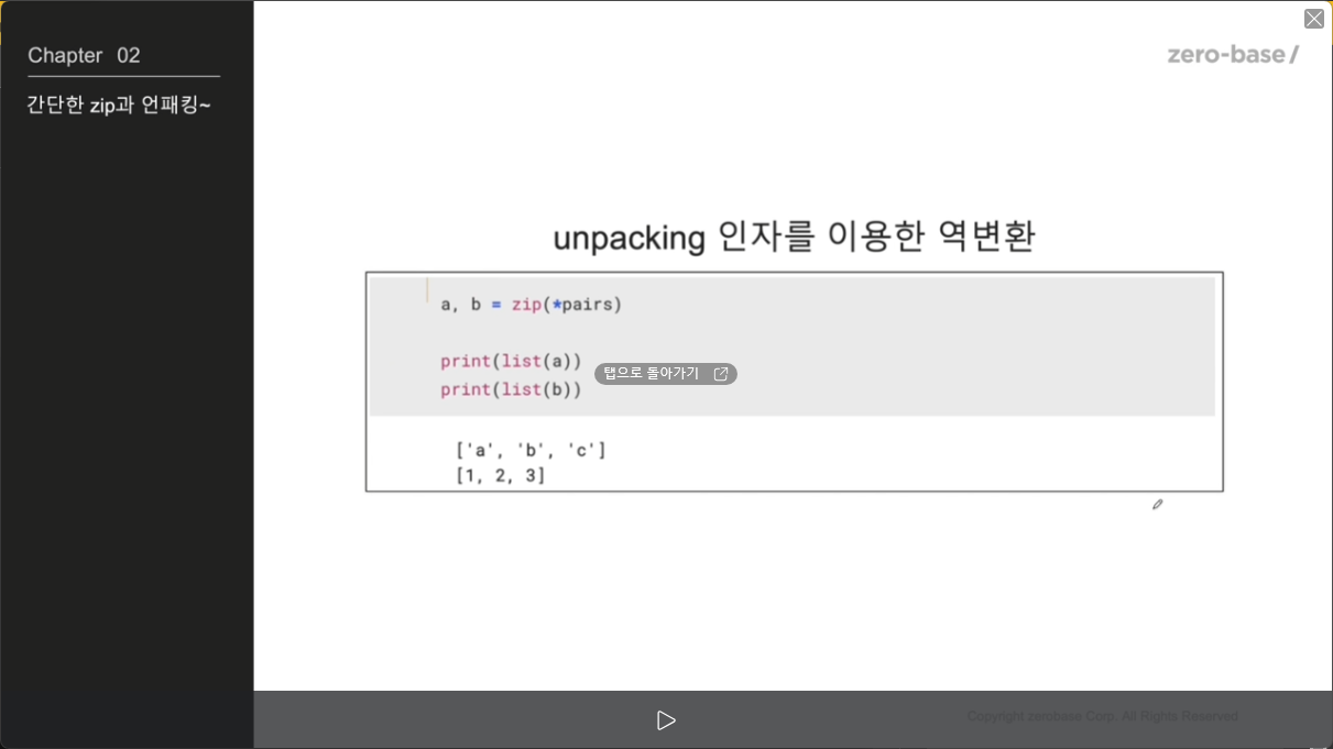
07 Decision Tree를 이용한 Iris 분류 - zip과 언패킹