
Decision Tree(결정트리)
- 분류, 회귀, 다중출력 작업에 활용가능한 머신러닝 알고리즘
- 강력한 머신러닝 알고리즘 중 하나인 랜덤포레스트의 기본 구성 요소
Decision Tree의 장점
- 데이터 전처리가 거의 필요하지 않다.
- 매우 직관적이고 결정 방식을 이해하기 쉬운 화이트 박스(white box) 모델이다.
사이킷런의 Decision Tree
- 사이킷런은 이진트리만 만드는 CART 알고리즘을 사용한다.
- CART알고리즘은 greedy algorithm으로 최적의 솔루션을 보장하지는 않는다.
CART 의 비용함수
훈련 데이터 세트를 하나의 특성 k와 그에 해당하는 임계값 t를 기준으로 두개의 subset으로 나눈다. CART함수의 비용함수는 두개의 subset의 불순도의 가중평균으로 모든 가능한 (k, t)들중 이 비용함수를 최소화할 수 있는 (k, t)를 찾으면 된다.
from sklearn.datasets import load_iris

from sklearn.preprocessing import StandardScaler
from sklearn.model_selection import train_test_split
from sklearn.metrics import accuracy_score
from sklearn.tree import DecisionTreeClassifier
from sklearn.tree import plot_tree

import matplotlib.pyplot as plt
iris 데이터셋 사용
iris=load_iris()iris.feature_names['sepal length (cm)',
'sepal width (cm)',
'petal length (cm)',
'petal width (cm)']iris.target_namesarray(['setosa', 'versicolor', 'virginica'], dtype='<U10')Decision Tree 구축 및 plot_tree를 이용한 시각화
x_train, x_test, y_train, y_test = train_test_split(iris.data, iris.target, test_size=0.2, random_state=1)
scaler = StandardScaler()
x_train = scaler.fit_transform(x_train)
x_test = scaler.transform(x_test)
model1 = DecisionTreeClassifier(criterion="entropy", max_depth=None, )
model1.fit(x_train, y_train)DecisionTreeClassifier(criterion='entropy')plt.figure(figsize=(12, 12))
plot_tree(decision_tree=model1, feature_names=iris.feature_names, class_names=iris.target_names, filled=True)
plt.show()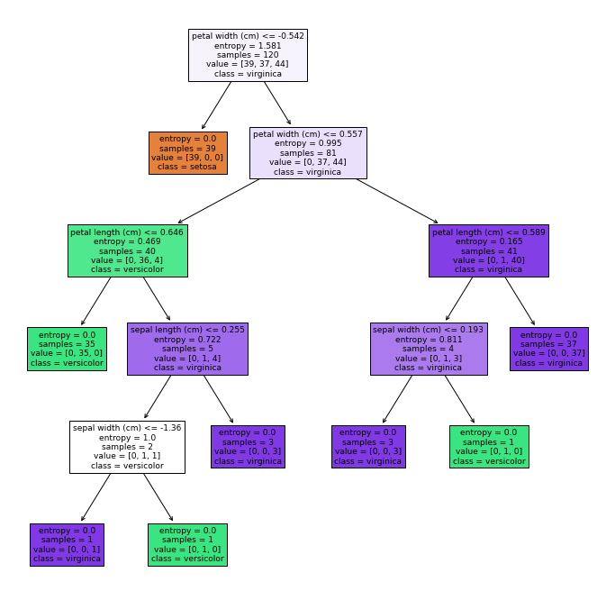
노드 살펴보기

- 루트 노드(root node): 깊이가 0인 맨 곡대기 노드
- 리프 노드(leaf node): 자식 노드를 가지지 않는 노드로 추가적인 조사를 하지 않는다.
- sample: 몇개의 훈련 샘플이 적용되었는지
- value: 각 클래스에 해당하는 훈련 데이터의 양
- class: 예측한 클래스 이름
which impurity method? gini vs entropy
- 둘중 어느것을 사용하든 실제로 큰 차이가 없다. 불순도 기준을 사용하여 트리를 평가하는데 시간을 들이는 것보다 가지치기(pruning) 방식을 바꿔보는 것이 더 낫습니다
- 지니 불순도가 로그를 계산할 필요가 없기 때문에 기본값으로 좋다.
- 엔트로피 방식이 조금 더 균형잡힌 트리를 만들 가능성이 높다.
Decision Tree의 단점
아래는 randomstate=2인 train data와 test data를 같은 비율이지만 다르게 나눈 동일한코드이다.
아래의 도식화된 그림을 보면 학습데이터에 변동이 최종결과에 큰 영향을 주는것을 알 수 있다.
x_train, x_test, y_train, y_test = train_test_split(iris.data, iris.target, test_size=0.2, random_state=2)
scaler = StandardScaler()
x_train = scaler.fit_transform(x_train)
x_test = scaler.transform(x_test)

model2 = DecisionTreeClassifier(criterion="entropy", max_depth=None) #깊이를 제안하는 파라미터 : max_depth
model2.fit(x_train, y_train)

plt.figure(figsize=(12, 12))
plot_tree(decision_tree=model2, feature_names=iris.feature_names, class_names=iris.target_names, filled=True)
plt.show()
Decision Tree Prunning
Decision Tree Clasifier의 max_depth의 조정으로 1 ~ max일때까지 test error를 통해 test error가 가장적은 노드를 기준으로 Prunning을 진행하였다.
max_depths = [depth+1 for depth in range(int(model1.get_depth()))]
max_depths
[1, 2, 3, 4, 5]train_error = []
test_error = []
for depth in max_depths:
model = DecisionTreeClassifier(max_depth=depth)
model.fit(x_train, y_train)
target_train_predict = model.predict(x_train)
target_test_predict = model.predict(x_test)
acc_train = accuracy_score(y_train, target_train_predict)
acc_test = accuracy_score(y_test, target_test_predict)
train_error.append(1-acc_train)
test_error.append(1-acc_test) plt.plot(max_depths, train_error, color="red")
plt.plot(max_depths, test_error, color="blue")
plt.show() {: width="60%" height="60%"}
위의 graph를 통해 파란색 test error을 보면 depth가 3일때 Prunning을 해야하는것을 알 수 있다.
model_f = DecisionTreeClassifier(criterion="entropy", max_depth=3)
model_f.fit(x_train, y_train)
DecisionTreeClassifier(criterion='entropy', max_depth=3)plt.figure(figsize=(12, 12))
plot_tree(decision_tree=model_f, feature_names=iris.feature_names, class_names=iris.target_names, filled=True)
plt.show()
위의 Decision Tree가 Pruning을 끝낸 최종 결과이다.
새로운 데이터에 대한 예측값과 예측확률
import numpy as np

new_data = np.array([[0.23, -0.87, 0.13, 0.9]])
print(model_f.predict_proba(new_data))
print(model_f.predict(new_data))
[[0. 0.25 0.75]]
[2]
study blog