논문 제목: Towards Real-Time Multi-Object Tracking
Introduction
현대의 Multiple Object Tracking(MOT)은 주로 'tracking-by-detection'의 방법을 따른다. 이 방법은 1) detection model, 2) appearance embedding model 두 개로 이뤄져있고, 이는 효율성의 문제를 발생시킨다. 이 방법을 Separate Detection and Embedding(SDE)라 논문의 저자들은 편의를 위해 명명했다.
연산량을 절약하기 위해 Faster R-CNN 구조를 채택한 방법이 있다. 이는 2-stage model로 RPN을 이용해 bounding box들을 detection 한 후 Fast R-CNN 부분의 classification 부분을 embedding model로 바꾼 구조를 이용한다. 2-stage model은 SDE보다 연산량을 줄였지만 여전히 10fps의 성능으로 real-time에 적용하기에는 무리가 있었다. 또한 target의 개수가 증가하는만큼 두번째 단계(embedding model)의 연산이 증가하는 문제가 존재한다.
본 논문은 MOT의 효율성을 증가시키기 위해 Jointly learns the Detector and Embedding(JDE)를 소개한다. 제안된 JDE는 하나의 network에서 동시에 detection 결과들과 이에 대응되는 appearance embedding들을 출력한다. JDE 방법은 SED 방법들과 비슷한 정확도를 보이면서 real-time 성능에 거의 근접했다. MOT-16 test set에 대해 20.2fps의 속도로 MOTA=64.4%를 이뤘다. 이에 비교해서 Faster R-CNN+ QAN embedding 모델은 6fps의 속도로 MOTA=66.1%를 보여줬다.
cf) MOTA란?
MOTA는 Multi-Object Tracking Accuracy를 의미하면 수식은 다음과 같다.
: the number of misses for time t
: the number of false positives for time t
: the number of mismatches for time t
: the number of all objects for time t
다음 사진1 은 SDE, Two-stage, JDE의 구조를 비교한 그림이다.
 사진 1. Model Comparison
해당 논문의 기여는 다음과 같다.
- Single-shot framework for joint detection and embedding learning인 JDE를 소개한다. 이는 state-of-the-art의 SDE와 유사한 정확도를 갖으면서 real-time 실행이 가능하다.
- Training data, network architecture, learning objectives and optimization strategy의 다양한 관점에 대해 분석하고 실험하여 JDE 구조를 설계했다.
- 같은 학습 데이터를 이용한 실험에서 JDE가 가장 빠른 속도를 달성하면서 SED 모델 조합들과 비슷한 성능을 보여줬다.
- MOT-16 데이터에서의 실험에서 training data의 수, accuracy, speed 의 이점을 JDE에서 확인할 수 있었다.
Joint Learning of Detection and Embedding
1. Problem Settings
JDE의 목적은 하나의 forward pass에서 location과 appearance embedding을 동시에 출력하는 것이다. 먼저 학습데이터 을 가정하자. 는 image frame을 나타내고, 는 하나의 프레임에서 k targets의 bounding box annotations를 나타낸다.는 label을 나타내고, -1인 경우 식별되는 label이 없는 즉 배경을 나타낸다. JDE는 예측된 bounding box들인 와 appearance embedding들인 를 출력하는 것을 목표로 한다. (이때, D는 embedding의 차원)
따라서 다음이 만족되어야 한다.
- is as class to as possible.
- Given a distance metric , that satisfy and , we have , where is a row vector from and , are row vector from , i.e., embeddings of targets in frame and , respectively
첫번째 목적은 target들을 정확하게 detect하는 것을 요구한다. 두번째 목적은 appearance embedding들에 대해 연속적인 frame에서 같은 label의 거리가 다른 label과의 거리 보다 작은 것을 요구한다. Distance metric은 Euclidean distance 또는 cosine distance가 될 수 있다.
2. Architecture Overview
 사진 2. Architecture
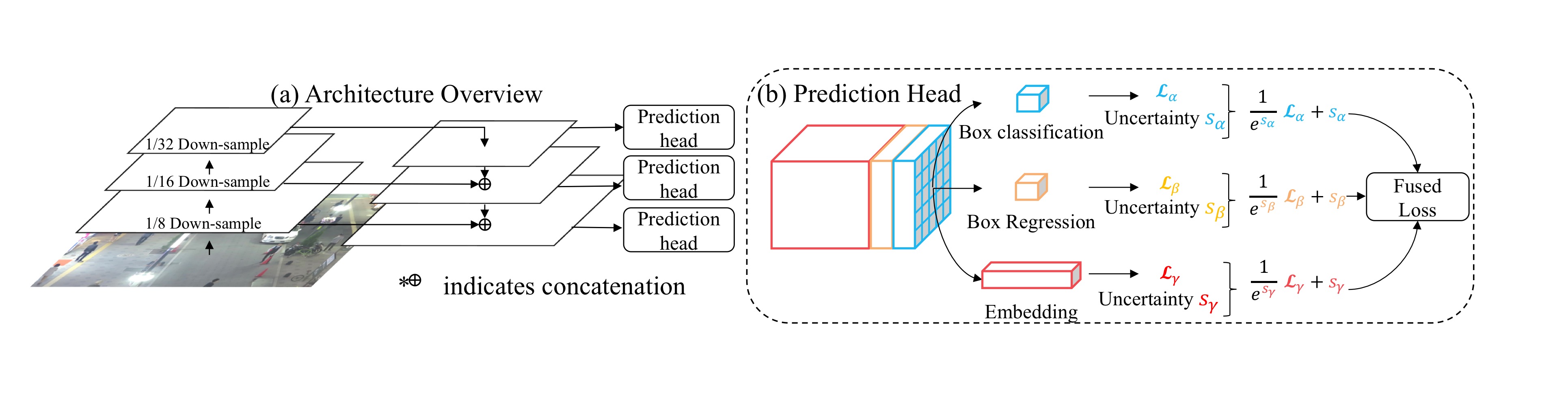
전체 구조는 Feature Pyramid Network(FPN)을 사용했고, 위의 사진2와 같다.
- Backbone network를 통해 3 scales feature map들을 얻는다.
- Feature map을 up-sampling한다. 이때 작은 feature map부터 순서대로 up-sample하면서 backbone network의 feature map을 skip-connection을 통해 concatenate하는 U-Net과 같은 구조를 갖는다.
- Up-sampling을 하면서 새롭게 얻은 3 scales feature map에 대해 각각 prediction head를 적용한다.
- Prediction head은 convolutional layer들로 구성되어 있고, (6A+D)xHxW의 dense prediction map인 output을 갖는다. (A는 anchor의 개수) Dense prediction map은 다음 3부분으로 나뉜다.
1) the box classification results of size 2A x H x W
2) the box regression coefficients of size 4A x H x W
3) the dense embedding map of size D x H x W
3. Learning to Detect
Detection branch는 Faster R-CNN의 RPN 구조와 유사하지만 2가지 변화를 줬다.
1) Anchors
보행자를 detect 하는 것이 목적이므로 aspect ratio를 1:3으로 고정했다. 또한 각각의 anchor의 scale을 부터 으로 해서 각 anchor에서 12개의 anchor box들을 사용한다.
2) Select foreground/background
Foreground(객체)와 background(배경) sample을 판별하기 위해 기존의 방법과 다른 threshold를 적용했다. Ground truth와 IoU가 0.5 이상인 경우 foreground로 하고, 0.4 이하인 경우 background로 했다. 이와 같은 기준은 시각화를 통해 결정했다.
Detection branch의 object function은 RPN과 같다. Foreground/ background classification을 위한 와 bounding box regression을 위한 가 있다.
: cross-entropy loss
: smooth-L1 loss
4. Learning Appearance Embeddings
같은 identity를 갖는 경우 가깝게 위치하고, 다른 identity를 갖는 경우 거리를 멀게 하는 embedding space를 학습하기 위해 triplet loss를 사용한다. triplet loss는 다음과 같다.
: instance in a mini-batch selected as an anchor
: positive sample
: negative sample
이러한 naive한 triplet loss를 사용할 때 몇 가지 문제가 존재한다.
1) Huge sampling space
첫번째 문제는 거대한 sampling space이다. positive sample과 negative sample을 모두 고려하는 경우 너무 큰 sampling space를 갖는다. 이를 해결하기 위해 hardest positive sample을 사용해 학습에 적용했다. Hardest positive sample은 positive sample 중에서 가장 positive라 예측하기 어려운 sample로 triplet loss에서는 거리가 가장 먼 sample이다. loss는 다음과 같이 변화한다.
2) Unstable and Convergence
Triplet loss를 사용한 학습은 불안정하고 수렴속도가 느릴 수 있다. 학습과정의 안정화와 수렴 속도를 빠르게 하기 위해서 smooth upper bound of triplet loss를 사용해 최적화를 진행한다.
위 식은 다음과 같이 표현할 수 있다.
이는 cross-entropy loss 공식과 유사하다.
: class-wise weight of the positive class
: class-wise weights of negative classes
와 의 구분되는 차이점은 2가지 이다.
- cross-entropy loss는 인스턴스 임베딩을 직접 사용하는 대신 학습 가능한 클래스 별 가중치를 클래스 인스턴스의 대리로 사용한다.
- cross-entropy loss는 embedding space를 고려해서 loss 계산 시 모든 negative sample들이 사용되는 반면에 upper loss의 경우 sampled negative instance들만을 사용한다.
위의 세 loss 중 어떤 loss를 사용할지 고려하고 실험적 결과로 논문의 저자들은 cross-entropy loss를 사용했다.
네트워크를 통해 추출된 embedding 벡터는 학습 시 shared fully-connected layer를 통해 class-wise logits가 된다. 그러고 나서 logits에 cross-entropy loss가 적용된다. Inference시에는 추출된 embedding 벡터를 사용해 객체를 추적한다.
5. Automatic Loss Balancing
: task-dependent uncertainty for each individual loss
: 번째 scale의 loss
: classification loss, bounding box regression loss, embedding loss
는 learnabel parameter로 학습시 자동으로 학습된다. 따라서 automatic loss balancing을 이루게 된다.
6. Online Association
본 논문의 주요 주제는 아니지만 논문의 저자들은 JDE와 함께 작동하는 간단하고 빠른 online association을 소개한다.
먼저 tracklet은 appearance state 와 motion state 로 표현된다. 여기서 는 bounding box center position, h는 bounding box height, 는 aspect ratio, 는 방향으로 velocity를 나타낸다.
-
tracklet appearnace 는 첫 번째 observation의 appearance embedding인 으로 시작된다.
-
observation들이 연관 될 가능성이 있는 모든 reference tracklet들을 포함하는 tracklet pool을 유지한다.
-
들어오는 프레임에 대해서 pair-wise motion affinity(유사성) matrix 과 appearnace affinity matrix 를 모든 observation들과 pool의 tracklet들에 대해서 계산한다. 이때 appearance affinity는 cosine similarity를 사용하고, motion affinity는 mahalanobis distance를 사용해 계산한다.
-
이후 선형 할당 문제를 cost matrix 인 Hungarian algorithm을 이용해 해결한다.
-
motion state는 Kalman filter에 의해 update되고, appearance state는 다음 수식으로 업데이트 된다.
where is the appearance embedding of the current matched observation, is a momentum term
-
마지막으로 어떤 tracklet들에도 할당 되지 않은 observation은 새로운 tracklet들로 시작된다. 또한 만약 최근 30 frame에서 update가 되지 않은 경우 tracklet은 종료된다.
논문에서 제안 online association은 SORT 보다 좋은 성능을 보여준다. 실험결과는 다음 사진3 과 같다.
 사진 3. comparison online association
Experiments
 사진 4. comparison of embed.loss & weighting strategy
위의 사진4를 통해 위에서 설명한 것과 같이 embedding loss로 cross-entropy를 사용할 때 성능이 가장 좋았고, 또한 weighting strategy도 automatic balancing을 통해 uncertainty를 이용한 모델이 성능이 가장 좋았다.
 사진 5. comparison with SOTA methods
위의 사진5를 통해 당시 SOTA의 object tracking 방법들과 비교했을 때 준수한 성능을 보여주면서 굉장히 빠른 속도를 확인할 수 있다.
Conclusion
해당 논문에서는 detection과 embedding을 함께 수행하는 JDE를 제안했다. 해당 모델은 당시 SOTA의 방법들과 비교했을 때 준수한 성능을 보이면서 real-time에 가까운 속도를 보여줬다.
후속 연구
FairMOT
논문 제목: FairMOT: On the Fairness of Detection and Re-Identification in Multiple Object Tracking
다음과 같은 문제점들을 해결하기 위해 제안된 논문이다.
- Unfairness Caused by Anchors: 동일한 객체에 여러 개의 anchor box들로 인해 Re-ID시 모호성이 생긴다.
- Unfairness Caused by Features: low-level feature와 high level feature를 동시에 학습시켜야 한다.
- Unfairness Caused by Feature Dimension: high-level feature를 학습하는 것이 object detection 성능에는 악영향을 미칠 수 있다. 또한 overfitting의 문제가 있다.
다음 사진을 통해 기존의 anchor-based model과 anchor-free model인 FairMOT의 차이를 확인할 수 있다.
 사진 6. Anchor base vs Anchor free
 사진 7. FairMOT Architecture
Backbone network은 ResNet-34를 채택한 Deep Layer Aggregation(DLA)를 이용하므로 multi-layer features들을 포착한다.
Detection branch에서 classification이 아닌 pixel-wise logistic regression을 통해 heatmap을 사용한다.
 사진 7. FairMOT performance
위의 사진7을 통해 대부분의 benchmark에서 state-of-the-art의 성능을 보여준다.
References
Towards Real-Time Multi-Object Tracking 논문: https://arxiv.org/abs/1909.12605
FairMOT 논문: FairMOT: On the Fairness of Detection and Re-Identification in Multiple Object Tracking
MOTA 관련 논문:
https://cvhci.anthropomatik.kit.edu/~stiefel/papers/ECCV2006WorkshopCameraReady.pdf
