
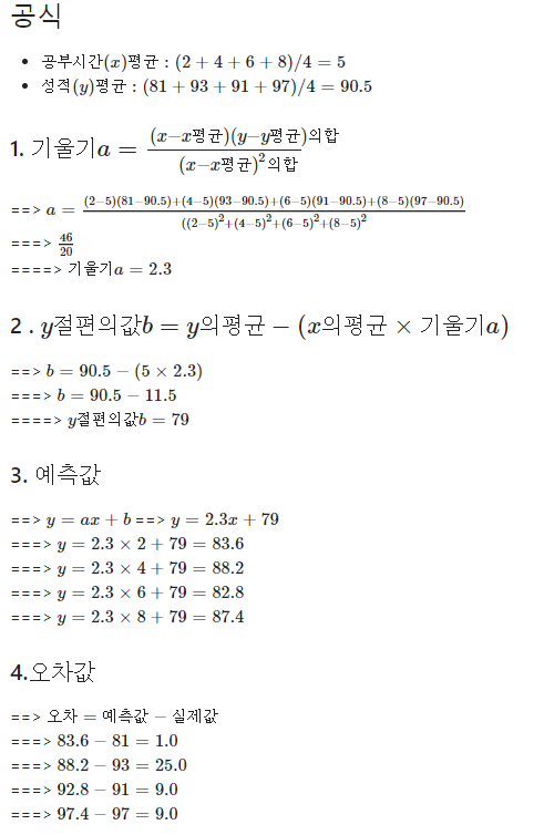
공부시간과 성적의 관계
| 공부시간 | 성적 | 예측값 |
|---|---|---|
| 2 | 81 | 83.6 |
| 4 | 93 | 88.2 |
| 6 | 91 | 92.8 |
| 8 | 97 | 97.4 |
fake_a_b는 임의의 예측값을 넣으면된다
아래는 공식으로 순차적으로 풀기위해
기본에서 계산처리한값들
# In[1]:
import numpy as np
import matplotlib.pyplot as pl
fake_a_b = [2.3, 79.0]
data = [[2, 81], [4, 93], [6, 91], [8, 97]]
## i[0]은 첫번째값(a), i[1]은 두번째값(y)
x = [i[0] for i in data]
y = [i[1] for i in data]
print("x => ", x)
print("y => ", y)
# In[2]:
## y = ax + b 에 대한 결과 처리 함수, EX) 예측값A * X값 + 예측값B = 3 * 2 + 76
def predict(x):
return (fake_a_b[0] * x) + fake_a_b[1]
# In[3]:
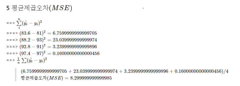
## MES 평균제곱오차, EX) Y값 점수 - 예측값, 81 - 82 = 1,0 = 1,0 * 1,0 = 1.0
def mse(y, y_hat):
return np.mean(((y - y_hat) ** 2))
# In[4]:
# MSE 평균오차 값
def mse_val(y, preidct_res):
return mse(np.array(y), np.array(predict_res))
# In[5]:
# 예측값 배열
predict_res = []
for i in range(len(x)):
predict_res.append(predict(x[i]))
print("시간 : ", x[i],
" 성적 : ", y[i],
" 예측값 : ", predict_res[i],
" 오차값 : ", mse(y[i], predict_res[i])
)
# In[6]:
print("MSE 값 : ", mse_val(y, predict_res))
# In[7]:
# 그래프 처리
pl.plot(x, y, label='BASE')
pl.scatter(x, y)
pl.plot(x, predict_res)
pl.scatter(x, predict_res)
pl.legend()
pl.show()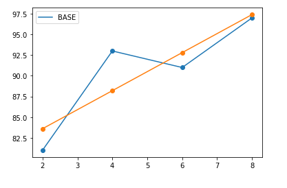

I will do, what i want!!