원문
1. Abstract
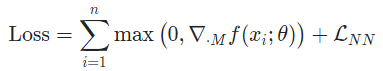
Monotonicity(단조성)은 현실 세계에서도 많이 요구되는 특성(제약) 중 하나이다. Monotonic Fully-Connected Neural Network를 구성하는 고전적인 방법으로는 가중치의 부호를 제한하는 방법이 있는데(증가하길 원한다면 양수, 감소하길 원한다면 음수), 이는 Activation Function으로 Sigmoid 함수를 사용하면 함수를 잘 근사하지 못하고, ReLU를 사용하면 Convex 함수만 잘 근사하는 문제가 있다. 이를 극복하고자 가중치의 부호를 제한하는 아이디어에 새로운 Activation Function을 도입하여 기존 방법들의 한계를 해결하고자 한다. 제안된 방법은 기존 방법들보다 (조금) 더 나은 성능을 보임과 동시에 월등히 적은 파라미터 수, 학습과정 변화의 불필요성, Universality 만족 등의 성과를 이루어냈다.
2. Background
2-1. Monotonic Architecture - by Construction
지금까지 Monotone Neural Network를 구현하기 위해 어떤 방법들이 제안되었는지 간단히 알아보자. Monotone Neural Network는 뜻 그대로 Monotonicity를 갖는 Neural Network를 말한다. 만약 입력출력이 모두 1차원이라면 Monotone Neural Network는 증가함수 또는 감소함수가 될 것이며, 다차원의 경우에도 모든 출력 성분이 각 변수에 대해 증가함수 또는 감소함수(=Partially Monotonically Increasing/Decreasing)가 될 것이다. 편의 상 증가함수에 대해서만 이야기하도록 하자.
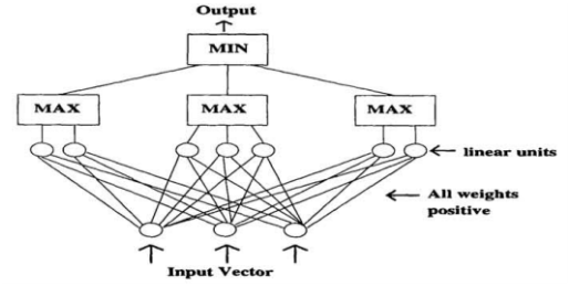
모든 Weight를 0 이상으로 제한 (Archer & Wang, 1993)
Fully Connected Neural Network의 모든 Weight를 0 이상으로 두어 증가함수를 표현할 수 있다. 기존의 Universal Approximation Theorem에 의해 임의의 함수를 표현하려면 음의 가중치가 반드시 필요했다. [1] 하지만 Sigmoid 함수나 Tanh 함수를 Activation Function으로 사용하면 본래 함수를 잘 추정하지 못했다고 한다.
이후 ReLU 함수가 대중적인 Activation Function으로 자리잡은 후, 위 방법에서 ReLU를 적용한 결과 Convex 함수만을 잘 추정할 수 있었다. 아핀 변환의 역할을 하는 nn.Linear과 ReLU 모두 Convex Function이므로, NN 자체가 Convex Function이 되기 때문이다.
그 외에도 다음 기법들이 고안되었다.
- 양의 가중치 & Max-Min Pooling (Sill, 1997)
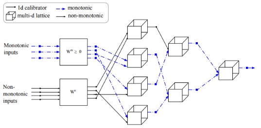
- Linear Calibrators & Lattice (You et al, 2017)
2-2. Monotonic Architecture - by Regularization
구조에서의 변화를 주는 대신, Regularization term을 이용해 Monotonicity를 보인 방법이 있다.
- Non Monotonicity에 페널티를 주는 항을 추가
- Soft Monotonicity Constraint를 추가한 Point Loss Function
- Monotonicity를 만족하지 않는 반례를 조정하며 학습
3. Main Idea
논문의 핵심 아이디어를 살펴보자. 그에 앞서 다음 개념을 정의한다.
3-1. Constrained Weight
Definition
다변수함수 가
을 만족시키면 는 partially monotonically increasing이다.
혹은
을 만족시키면 는 partially monotonically decreasing이다.
논문의 목표는 partially monotonically increasing/decreasing을 만족하는 Neural Network를 설계하는 것이다. 심지어 입력 데이터가 2차원 이상의 벡터인 경우, 각 변수마다의 증가/감소를 결정할 수 있다. [2]
Definition
-dimensional monotonicity indicator vector 을 다음과 같이 정의한다.
입력 변수마다의 증가/감소 여부는 monotonicity indicator vector 로 결정한다. 입력 벡터의 번째 변수가 증가하길 원한다면 , 감소하길 원한다면 , 증가/감소를 결정하고 싶지 않다면 을 부여한다.
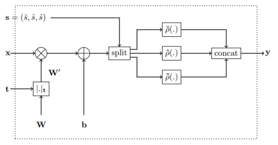
monotonicity indicator vector 가 결정되면 이를 이용하는 연산 를 다음과 같이 정의한다.
행렬 에 대하여 의 성분은
이다. [3] 이로부터 Fully-Connected layer는
로 정의되며, 이후 새로운 Activation Function을 적용한다.
Lemma 1은 Constrained Weight를 곱한 후 bias를 더하더라도 Monotonicity가 그대로 만족됨을 설명한다. 증명은 어렵지 않아 생략한다.
Lemma 1
각 에 대하여,
를 만족한다.
3-2. Activation Function
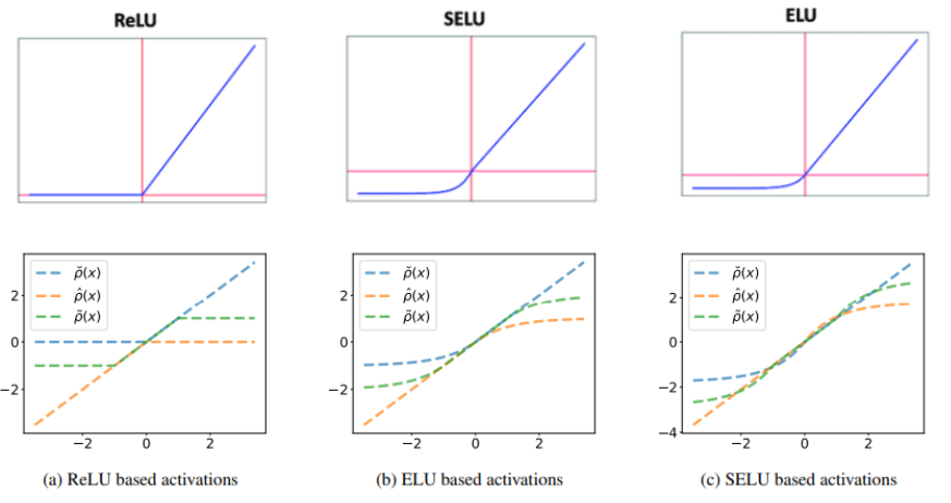
논문에서는 ReLU와 같은 Unbounded Activation Function을 활용할 방법을 제안하였다. Convex Function만을 추정할 수 있다는 한계를 극복하고자 다음과 같은 Activation Function을 정의하였다.
Definition
를 zero-centered, monotonically increasing, convex, lower-bounded 함수라 하자.
각 Activation Function은 다음과 같은 특징을 갖는다.
- : 원래 사용하려던 Activation Function (convex, lower-bdd)
- : 의 원점대칭 함수 (concave, upper-bdd)
- : 와 가 혼합된 함수 (non-convex, non-concave, bounded)
예를 들어, 를 ReLU, SeLU, ELU로 하였을 때의 는 다음과 같다.
세 Activation Function을 통합하여 Activation Function 를 정의한다.
Definition
를 zero-centered, monotonically increasing, convex, lower-bounded 함수라 하고, , , 이라 하자.
Activation Function 을 다음과 같이 정의한다.
즉, 는 아핀 변환 이후의 벡터를 차례로 개씩 나누어 각각 를 적용하는 것이다. 각 함수에 몇 개의 성분을 할당하냐에 따라 convex, concave의 정도가 달라질 것이다. Corollary 3은 이러한 Activation Function이 Monotonicity를 해치지 않음을 이야기한다.
Corollary 3
라 하자. 각 에 대하여,
를 만족한다.
지금까지의 과정을 다음 그림과 같이 나타낼 수 있다. 이를 Monotonic Dense Block이라 부른다.
4. Architecture
Monotonic Dense Block을 여러 개 이어붙여 네트워크 아키텍쳐를 구성할 수 있는데, 논문에서는 크게 2가지 타입을 소개한다.
-
Type1
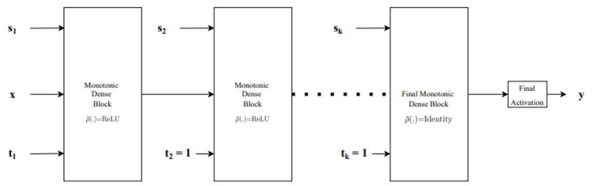
Monotonic Dense Block을 단순히 이어붙인 구조다.- 2번째 블록부터 monotonicity indicator vector 가 항상 벡터이다. 변수의 증가/감소 여부는 첫 번째 블록에서 결정되고, 이후 블록에서는 항상 증가함수를 합성함으로써 증가/감소를 유지한다.
- 마지막 블록의 Activation Function은 Identity를 사용한다. 만약 이라면 bounded Activation Function이 합성되어, Neural Network로 나타낼 수 있는 함수가 크게 제한되기 때문이다.
-
Type2
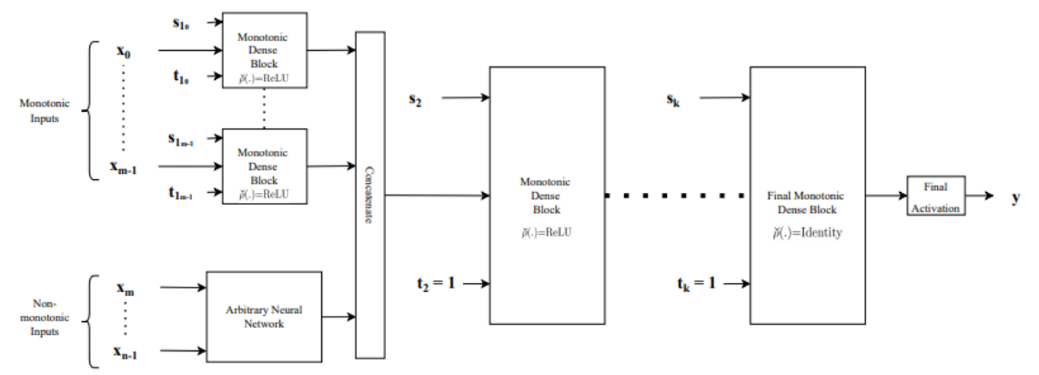
입력 벡터가 Monotonic/Non-Monotonic으로 나누어져 네트워크를 통과하는 구조다.- Monotonic Inputs은 각 변수의 증가/감소를 결정할 수 있다. 각 변수마다의 convex/concave를 결정할 수 있도록 하기 위해 개별적인 Monotonic Dense Block을 사용한다.
- Non-Monotonic Inputs은 일반적인 Neural Network를 통과한다. Feature Extracting 등 Neural Network의 역할을 목적에 맞게 부여할 수 있다.
- 두 Input이 concatenate되어 다시 Monotonic Dense Block을 통과한다. Type1과 마찬가지로 monotonicity indicator vector 가 항상 벡터로 고정되며, 마지막 블록의 Activation Function으로 Identity를 사용한다.
5. Universality
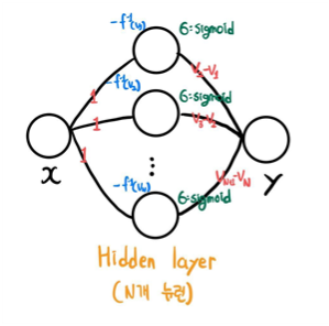
지금까지 Monotone Neural Network의 구조를 살펴보았다면, 이러한 구조가 실제로 임의의 Monotone Function을 잘 근사할 수 있는지에 대한 이론적 근거가 필요하다. Theorem 4는 Sigmoid 함수를 Activation Function으로 사용하였을 경우에 대한 이론적 근거를 제시한다. [4]
Theorem 4 [5]
임의의 continuous, monotone nondecreasing 함수 에 대하여, 다음을 만족하는 feedforward neural network가 존재한다.
- 최대 개의 hidden layer
- sigmoid를 Activation Function으로 사용
- 양의 가중치
- 임의의 와 에 대하여 을 만족하는 벡터 를 출력
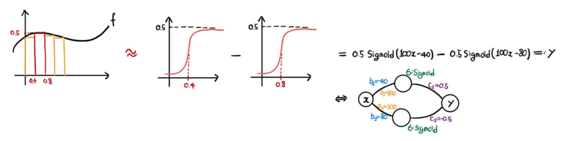
우리의 목적은, [5]에서 사용된 Heavyside Function 를 로 대체하는 것이다. Lemma 5는 가 를 이용하여 표현할 수 있음을 주장한다.
Lemma 5
를 zero-centered, monotonically increasing, convex, lower-bounded 함수라 하자. 함수
는 에서 함수
로 근사될 수 있다.
또한 Lemma 6은 를 로 대체할 수 있음을 주장한다.
Lemma 6
어떤 에 대하여, Activation Function 가
를 만족한다고 하자.
를 Activation Function으로 사용하는 모든 constrained monotone neural network 에 대하여
를 만족하는, 를 Activation Function으로 사용하는 constrained monotone neural network 이 존재한다.
즉 는 로 근사할 수 있으며, 를 Activation Function으로 사용하는 Neural Network 를 로 똑같이 만들 수 있다는 흐름이다.
이로부터 Theorem 7은 Constrained Monotone Neural Network의 이론적 근거를 제시한다.
Theorem 7
를 zero-centered, monotonically increasing, convex, lower-bounded 함수라 하자. compact set 에서 정의된 임의의 multivariate continuous monotone 함수는 다음을 만족하는 monotone constrained neural network로 근사될 수 있다.
- 최대 개의 hidden layer
- 를 Activation Function으로 사용
Theorem 7은 최대 hidden layer의 수 역시 제시하지만, 실험에 의하면 그보다 적은 개수를 사용하였을 때 더 좋은 성능을 보였다고 한다.
6. Experiment
논문은 기존의 Monotone Neural Network와 성능을 비교한 실험을 진행하였다. 3개의 데이터셋 COMPAS, Blog Feedback, Loan Defaulter 모두에서 최소 파라미터 수와 최고 성능을 달성하였다.
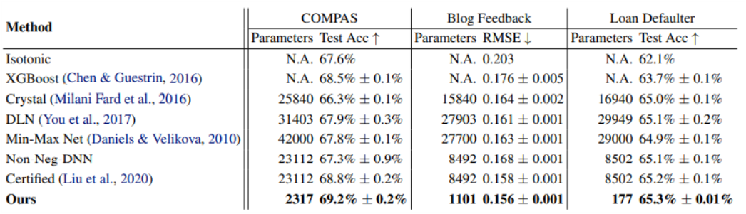
- COMPAS : 13개의 Feature 중 4개의 Monotone Feature를 가진 분류 문제
- Blog Feedback : 276개의 Feature 중 8개의 Monotone Feature를 가진 회귀 문제
- Loan Defaulter : 28개의 Feature 중 5개의 Monotone Feature를 가진 분류 문제
또한 Monotone Feature만을 가진 데이터셋에 대해서도 최고성능을 달성하였다.
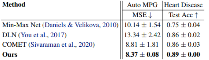
- AutoMPG : 3개의 Monotone Feature를 가진 회귀 문제
- Heart Disease : 2개의 Monotone Feature를 가진 분류 문제
7. Code
이곳에서 Colab 코드를 제공하고 있다. 지금은 이변수함수 를 근사하는 Monotone Neural Network를 학습시켜보자.
데이터 생성
에 노이즈를 섞은 학습 데이터를 생성한다.
import numpy as np
import pandas as pd

rng = np.random.default_rng(42)


def generate_data(no_samples: int, noise: float):
    x = rng.normal(size=(no_samples, 2))
    y = x[:, 0] ** 3
    y += np.exp(-x[:, 1])
    y += noise * rng.normal(size=no_samples)
    return x, y


x_train, y_train = generate_data(10_000, noise=0.1)


d = {f"x{i}": x_train[:5, i] for i in range(2)}
d["y"] = y_train[:5]
pd.DataFrame(d).style.hide(axis="index")
모델 구성
패키지를 설치하여 MonoDense는 Monotone Dense Block을 이용할 수 있다. 이를 Sequential에 쌓아 모델을 구성한다.
!pip install monotonic-nn

from tensorflow.keras import Sequential
from tensorflow.keras.layers import Dense, Input

from airt.keras.layers import MonoDense

model = Sequential()

model.add(Input(shape=(2,)))
monotonicity_indicator = [1, -1]
model.add(
    MonoDense(128, activation="elu", monotonicity_indicator=monotonicity_indicator)
)
model.add(MonoDense(128, activation="elu"))
model.add(MonoDense(1))

model.summary()
모델 학습
learning rate, optimizer 등을 설정하고 모델을 학습시킨다.
from tensorflow.keras.optimizers import Adam
from tensorflow.keras.optimizers.schedules import ExponentialDecay

lr_schedule = ExponentialDecay(
    initial_learning_rate=0.01,
    decay_steps=10_000 // 32,
    decay_rate=0.9,
)
optimizer = Adam(learning_rate=lr_schedule)
model.compile(optimizer=optimizer, loss="mse")

model.fit(
    x=x_train, y=y_train, batch_size=32, validation_data=(x_val, y_val), epochs=10
)
결과 확인
학습 결과를 정답과 비교하며 확인한다.
import matplotlib.pyplot as plt
from mpl_toolkits.mplot3d import Axes3D

fig = plt.figure(figsize=(9, 6))
ax = fig.add_subplot(111, projection='3d')
x_val, y_val = generate_data(100, noise=0.0)
pred = model.predict(x=x_val)

x = x_val[:, 0]
y = x_val[:, 1]
z1 = pred[:, 0]
z2 = y_val

ax.scatter(x, y, z1, color = 'r', alpha = 0.5)
ax.scatter(x, y, z2, color = 'g', alpha = 0.5)
# 예측 : red
# 정답 : greed
결과는 다음과 같다.
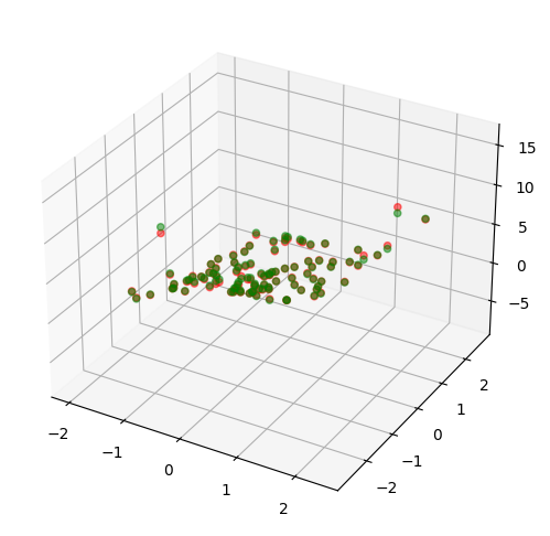
붉은 점과 초록 점이 잘 포개어진 것으로 보아, 학습이 잘 되었음을 알 수 있다. 또한 축, 축 별로 grid 데이터를 생성하여 변수 별 Monotonicity를 검증할 수 있다.
8. Conclusion
이 논문은 Monotonicity를 보장하는 Neural Network의 구현 및 Universality 달성을 주장하며 다음 3가지를 특징으로 뽑는다.
- Fully-Connected layer를 즉시 Monotone Dense Block으로 대체 가능
- 기존 네트워크의 layer와 구조적으로 차이가 없다는 점이다. 이는 Monotone Dense Block의 범용성과 확장성을 강조한다.
- 성능을 유지하면서 압도적으로 적은 파라미터 수
- 실험 결과 기존 모델에 비해 최고 성능을 달성했지만, 큰 차이를 보이지 못했다. 하지만 압도적으로 적은 파라미터 수를 사용하면서, 학습속도 및 연산량에서 큰 장점을 보였다.
- Convolution layer 등 다른 유형의 layer와의 연계 기대
- 현재는 Type2 Architecture와 같이 Fully-Connected layer와 함께 사용하였지만, 적절한 변형을 통해 Convoulution layer와 같은 다양한 layer와 함께 사용될 수 있기를 기대할 수 있다.
Endnotes
[1] 아주 작은 구간에서만 0이 아닌 값을 갖는 막대 모양의 함수를 만들기 위해선, Sigmoid 모양의 함수를 빼서 만들어야 한다.
[2] 예를 들어 입력이 인 이변수함수 를 근사하고자 할 때, 에 대해서는 증가, 에 대해서는 감소하도록 하는 Neural Network를 설계할 수 있다.
[3] 입력 데이터 , monotonicity indicator vector 와 다음 초기 가중치 행렬() 로 예를 들어보자.
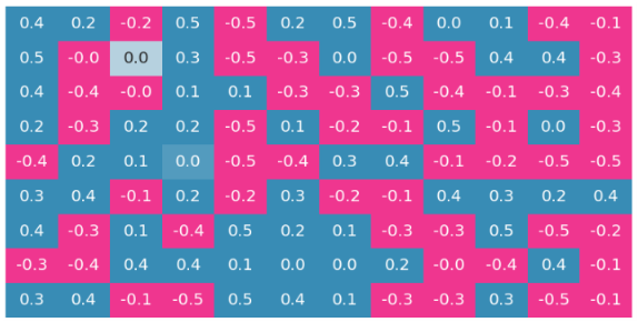
앞선 세 변수는 감소, 중간 세 변수는 증가/감소에 제약이 없으며, 마지막 세 변수는 증가하도록 네트워크를 구성하는 과정이다. 에 의한 연산 결과 는 다음과 같이
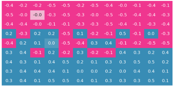
감소하는 세 변수와 곱해지는 1~3행은 음수(or ), 증가/감소 제약이 없는 변수와 곱해지는 4~6행은 기존과 그대로, 증가하는 세 변수와 곱해지는 7~9행은 양수(or )로 계산된다.
[4] 다만 Background에서 소개한 바에 의하면 Sigmoid를 Activation Function으로 사용하면 함수를 잘 근사하지 못한다. 이러한 모순점이 명확하게 해결되지 않는데, 이론적 근거는 충분하지만 실험에서 의미있는 결과를 얻지 못했다고 감히 추측해본다.
[5]
Theorem 4의 증명은 수학적 귀납법의 흐름으로 전개된다. 입력 벡터 에 대하여 일 때의 증명을 소개한다.
다음 두 가지를 가정한다.
- : strictly increasing
- ()
strictly increasing은 추후 increasing으로 확장 가능하며, compact set에서 연속인 는 bounded라는 사실로부터 lower bound 를 더해 로 만들 수 있다.
이로부터 를 Heavyside Function 를 이용하여 다음과 같이 나타낼 수 있다.
가 continuous, strictly increasing이므로 역함수가 존재하여
이고, 는 compact set에서 continuous이므로 리만 적분 가능하여
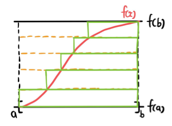
로 나타낼 수 있으며, 이는 다음과 같은 neural network로 나타낼 수 있다.