선형 회귀 모델: Basis Function

Yougurt_Man·2022년 4월 23일

Basis Function Linear Regression gaussian

Machine Learning Theory

목록 보기

5/18

Keywords

D-dimensional Linear Regression Model
Linear Combination
Basis Function
- Gaussian Basis
Loss Function with Gaussian (Utilizing MSE)
Analytical Solution with Gaussian (Code)

Note

Analytical vs Numerical Solution

Analytical Solution (해석해) - 정확한 해를 구함
Numerical Solution (수치해) - 근사치를 구함.

N-dimensional Linear Regression Model

입력 데이터와 출력 데이터가 선형관계일때 Linear Regression의 기본적인 선형함수는 다음과 같다.

(1) $y(x,w)=w_0x_0 + w_1x_1 + ...+ w_Nx_N$

하지만, 임의의 입력 데이터가 출력 데이터에 대해, 항상 선형적인 관계를 지닌다고 가정할 수 없다.

이때, X를 어떤 단계를 거쳐 비선형 데이터를 조작할 수 있는데 이를 Basis Function이라고 부른다.

Basis Function

Basis Function을 Wiki 문서에서 찾아보면,

In mathematics, a basis function is an element of a particular basis for a function space. Every function in the function space can be represented as a linear combination of basis functions, just as every vector in a vector space can be represented as a linear combination of basis vectors.

출처: https://en.wikipedia.org/wiki/Basis_function

Basis Function이란, 함수 공간을 구성하는 기본 원소이며, 임의의 연속함수 ( $\in$ Function Space)는 Basis Function의 선형 결합으로 표현할수 있다. * Basis Vector의 선형 결합으로 공간을 Span하는 Vector Space의 개념과 유사하다.

이를 확장해서, 우리가 구하려는 함수 값 $y(x,w)$ 와 Basis Function인 $\phi(x)$ 가 함수공간 $R^n$ 을 생성한다면, 입력 데이터 x를 Basis Function $\phi(x)$ 의 선형 결합으로 $y$ 를 표현할 수 있다는 뜻이 된다.

이를 (1) 식에 적용 시키면,

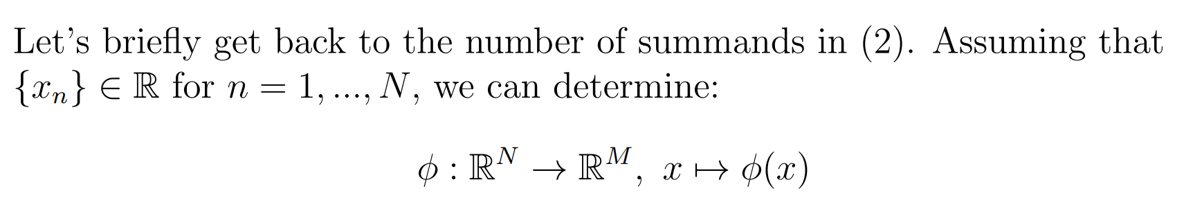
(2) $y(x,w) = w_0 + w_1\phi_1(x) + ... w_m\phi_{D-1}(x)$

(3) $y(x,w) = w_0 + \displaystyle\sum_{j=0}^{d-1}w_j\phi_j(x)$

만약, $\phi_0(x)$ = 1 라는 더미 함수를 사용하게 되면 (3)을 간단하게 표현할 수 있다.

(4) $y(x,w) = \displaystyle\sum_{j=0}^D w_j\phi_j(x) = w^T\phi(x)$

$w = (w_0, w_1,...w_D)$
$\phi = (\phi_0, \phi_1, ... , \phi_D)$

주목할 점은, (1) 식이 가지는 D != N의 특징 벡터를 다루는 함수식의 개수가 다르다. 데이터의 차원이 기저함수 $\phi(x)$ 를 로 Transformation이 있었다는것을 의미하는 것 같다. 아래 설명에 따르면, Basis Function $\phi$ 는 입력 벡터 $X$ 를 실수공간 $\R^N \rightarrow \R^M$ 차원으로 확장하고, 함수값 y가 가중치 $w$ 와 $\phi(x)$ 에 대해 Linear 한것을 보여준다.

출처: Linear.Models.for.Regression_Handout_Nadia.pdf

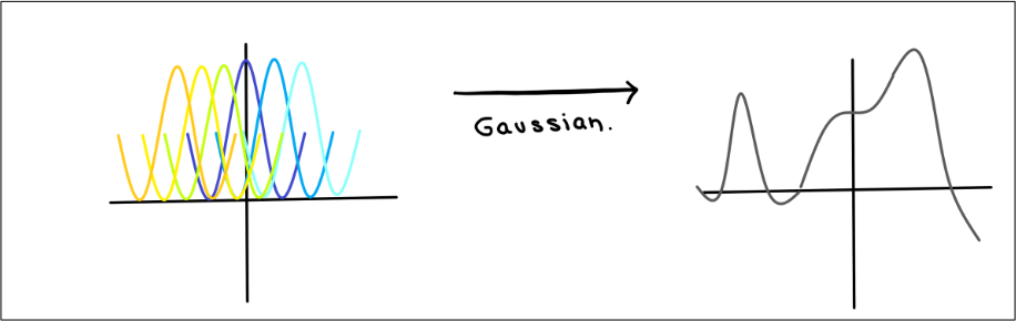
Gaussian Basis Function

Basis Function의 종류로 Gaussian Basis Function을 알아보자.

The graph of a Gaussian is a characteristic symmetric "bell curve" shape

출처: https://en.wikipedia.org/wiki/Gaussian_function

Gaussian Function은 함수의 중심을 기준으로 Symmetric (대칭)한 특성으로 그래프가 Bell Curve 형태를 가진다.

출처: Linear.Models.for.Regression_Handout_Nadia.pdf

Gaussian Basis Function 의 그래프는, 평균(Mean)을 의미하는 $\mu$ 와 Standard Deviation을 의미하는 $\sigma$ 에 의해 결정되며 다음과 같은 함수식을 나타낸다.

$\phi_j(x) = a * exp{-(x-\mu_j)^2 \over 2s^2}$

$a$ : Height of Graph
$j$ : Index
$mu_j$ : Mean (평균, 함수의 중심을 나타냄)
$\sigma$ : Standard Deviation (표준편차)
$\sigma^2$ : Variance (분산).

Gaussian Basis Function을 간단히 코드로 구현해보자

# 가우스 기저 함수 구현하기 

from IPython.core.pylabtools import figsize
plt.figure(figsize = (5,5))

plt.grid(True)

input_data = np.linspace(0,11, 100)
center = np.mean(input_data) 
standard_dev = 
a = 2 # Determines the height of graph 
print(center) # This is the only point what I would like to give different color
gauss_function = a * np.exp(-((input_data-center)**2)/standard_dev**2)
plt.plot(input_data, gauss_function)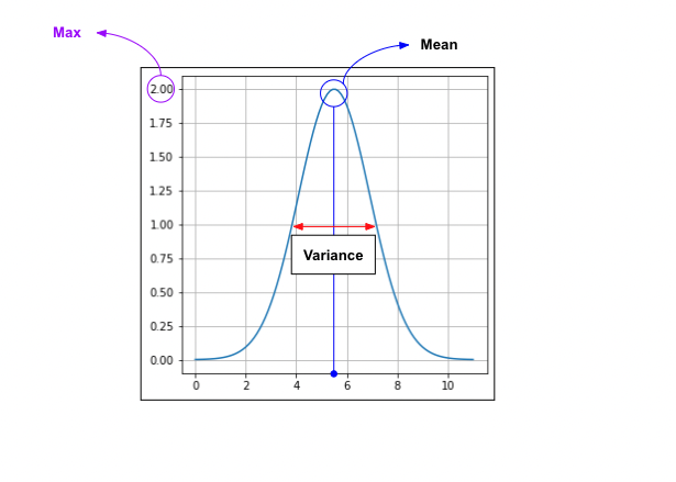

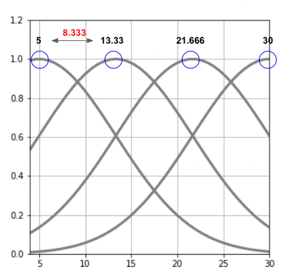
Gaussian Basis Function 그래프를, 여러개 그리는 코드는 다음과 같다.

def gauss(x, mu, s): 
  return np.exp(-(x-mu)**2 / (2*s**2)) 

# 4개의 가우스 함수 그리기 

M = 4 # 가우스 함수 개수 
plt.figure(figsize = (5,5))
mu = np.linspace(5,30, M) # 평균 >> 이게 왜 평균이 되지..? 
print(mu)
print(mu.shape)
# print(mu)
s = mu[1] - mu[0] # 인접한 가우스 함수 간 중심 사이의 거리 
print("Standard Deviation: {}".format(s)) # 가우스 함수간 거리는 8.333333
xb = np.linspace(x_min,x_max, 40) # ndarray로 100개의 value 저장 
print(type(xb)) # return type - numply.ndarray 

for j in range(M): # 4번 반복 
  y = gauss(xb, mu[j], s) # 
  print(y)
  plt.plot(xb, y, color='gray', linewidth=3)

print(y.shape)

plt.grid(True)
plt.xlim(x_min, x_max)
plt.ylim(0, 1.2)