Overview

Traffic Sign Detection is designed for a final term project on my first semister. The main goal of the project is to utilizing popular libraries and network algorithm structures: Tensor Flow, Keras, Pyplot and others.

Goal

• Build a Training Model using Keras library
• Utilize a ResNet50 Algorithm
• Classify a random given image

Operating Enviroment.

• Colab (Basic, GPU)
  • Training Time: ~57.321 Sec
• ResNet50V2
  • Features Transfer Learning
  • Better performance than an oridinaray ResNet50 algorithm
• DataSet: Sourced from Kaggle, Traffic-Sign-Classification-CNN-Official (https://www.kaggle.com/code/ahemateja19bec1025/traffic-sign-classification-cnn-official/data)

Code with Description.

Mount Google Drive

import glob 
from google.colab import drive

# Mount your google drive with your colab
drive.mount('/content/gdrive')

# Make directory in your content at content folder
! mkdir my_data

# Download dataset
!cp '/content/gdrive/MyDrive/정보과학대학원/전공/1학기/딥러닝과응용/Traffic Sign Detection/archive.zip' 'my_data'

# Unzip it into "my_data"
!unzip -n "/content/my_data/archive.zip" -d "/content/my_data" 

To bring a dataset into a colab enviroment, colab connects to google drive.

Loaded dataset will be located at /content/my_data/

Check lables

import pandas as pd 
# Read labels
labelfile = '/content/my_data/labels.csv'
pd.read_csv(labelfile)

Pandas helps to read csv formatted file.

index	ClassId	Name
0	0	Speed limit (5km/h)
1	1	Speed limit (15km/h)
2	2	Speed limit (30km/h)
3	3	Speed limit (40km/h)
4	4	Speed limit (50km/h)
...	...	...
54	54	No stopping
55	55	No entry
56	56	Unknown7
57	57	Unknown8

Show sample image

# Show sample images of each class 
from PIL import Image 
import os 
import os.path
import numpy as np
import matplotlib.pyplot as plt 
%matplotlib inline

root_path = "/content/my_data/traffic_Data/DATA"

get_dir = os.listdir(root_path)

Preprocess images

# Preprocessing Image
# - Referenced: https://colab.research.google.com/github/tensorflow/docs/blob/master/site/en/tutorials/images/classification.ipynb#scrollTo=fIR0kRZiI_AT
from tensorflow.keras.preprocessing import image_dataset_from_directory
from tensorflow.keras.preprocessing.image import ImageDataGenerator, load_img, img_to_array

bat_size =  64
img_height = 32
img_width = 32

train_ds = image_dataset_from_directory(
    directory= root_path,
    labels='inferred',
    label_mode='int',
    batch_size=bat_size, 
    image_size = (img_width,img_height), # Fix Image Size
    validation_split=0.2,
    seed= 123,
    subset="training"
)

validation_ds = image_dataset_from_directory(
    directory= root_path,
    labels='inferred',
    label_mode='int',
    batch_size=bat_size,
    image_size = (img_width,img_height),
    validation_split=0.2,
    seed= 123,
    subset="validation"
)

Generate dataset into train_ds for training, validation_ds for validation with image_dataset_from_directory provided by Tensorflow.

Found 4170 files belonging to 58 classes.
Using 3336 files for training.
Found 4170 files belonging to 58 classes.
Using 834 files for validation.

Rescale Image

Due to the large scale of image pixel value, range from 0 to 255, rescaling the size of image is not an option, but necessary.

# Reduce the size of input to layers >> Standarize the data 
from tensorflow.keras import layers
normalization_layer = layers.experimental.preprocessing.Rescaling(1./255)

Build Model

ResNet50V2

ResNet50v2 is powerful algorithm for image training.

As the dataset has very limited data, Transfer Learning (Bring already-learnt bias and weights from other model) will be great option. In this case, ResNet50v2 is my choice.

resnet50 = tf.keras.applications.ResNet50V2(
    include_top=False,
    input_shape=(img_height,img_width,3),
    weights="imagenet",
    classes=num_classes,
    pooling='avg',
)

for layer in resnet50.layers:
  layer.trainable=False # Do not train again

Add layers

Build a sequential model by adding dense layers.

To keep away from overfitting, drop-out method will do.

model = Sequential()
# Before input the img to CNN, Rescaling may help reducing a learning time, and model performance. 
model.add(layers.experimental.preprocessing.Rescaling(1./255, input_shape=(img_height, img_width, 3)))
model.add(resnet50)
model.add(Flatten())
BatchNormalization() # Normalize 
model.add(Dense(2048, activation='relu'))
BatchNormalization() # Normalize 
layers.Dropout(0.2)
model.add(Dense(1024, activation='relu'))
BatchNormalization() # Normalize 
layers.Dropout(0.2)
model.add(Dense(num_classes))

compile model

learning_rate = 5e-5

optimizer = keras.optimizers.Adam(learning_rate=learning_rate)

model.compile(optimizer=optimizer, # Default Optimizer does not make good performance.
              loss=tf.keras.losses.SparseCategoricalCrossentropy(from_logits=True),
              metrics=['accuracy'])
model.summary()

Optimized learning rate is important to find optimized minimum. In this case, 5e-5 make a great performace in my case.

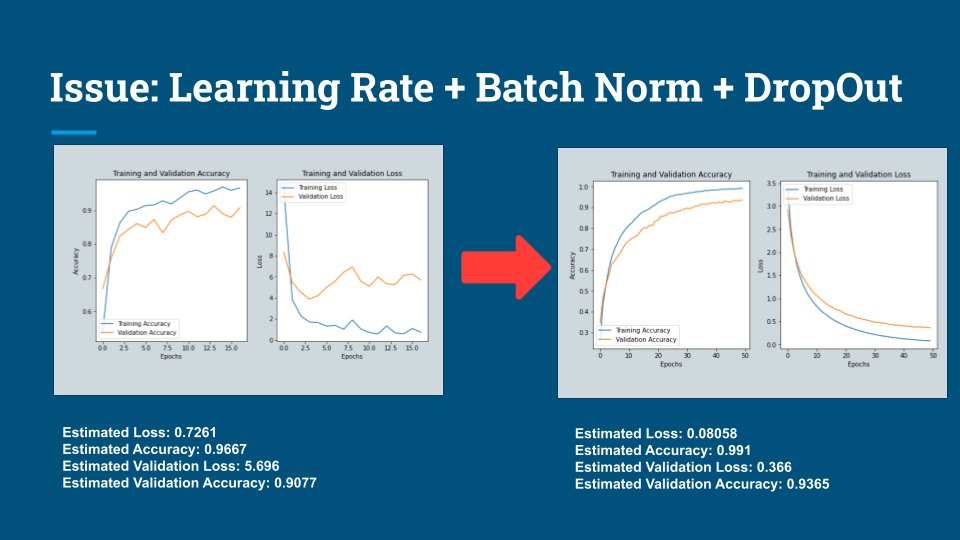
The following shows that Learning Rate + Batch Norm + Dropout improves model performance in terms of Accuracy / Loss

Train Model

import time

epochs=50

# Trigger the "Early Stopping" callback function if parameters is no longer needed to be learnt.

callback = tf.keras.callbacks.EarlyStopping(monitor='loss', patience=5, verbose=1)

Starting_Time = time.time()

print("Training Begin !")

history = model.fit(
  train_ds,
  validation_data=validation_ds,
  epochs=epochs,
  callbacks=[callback] # Call Early Stopping 
)
End_Time = time.time() - Starting_Time
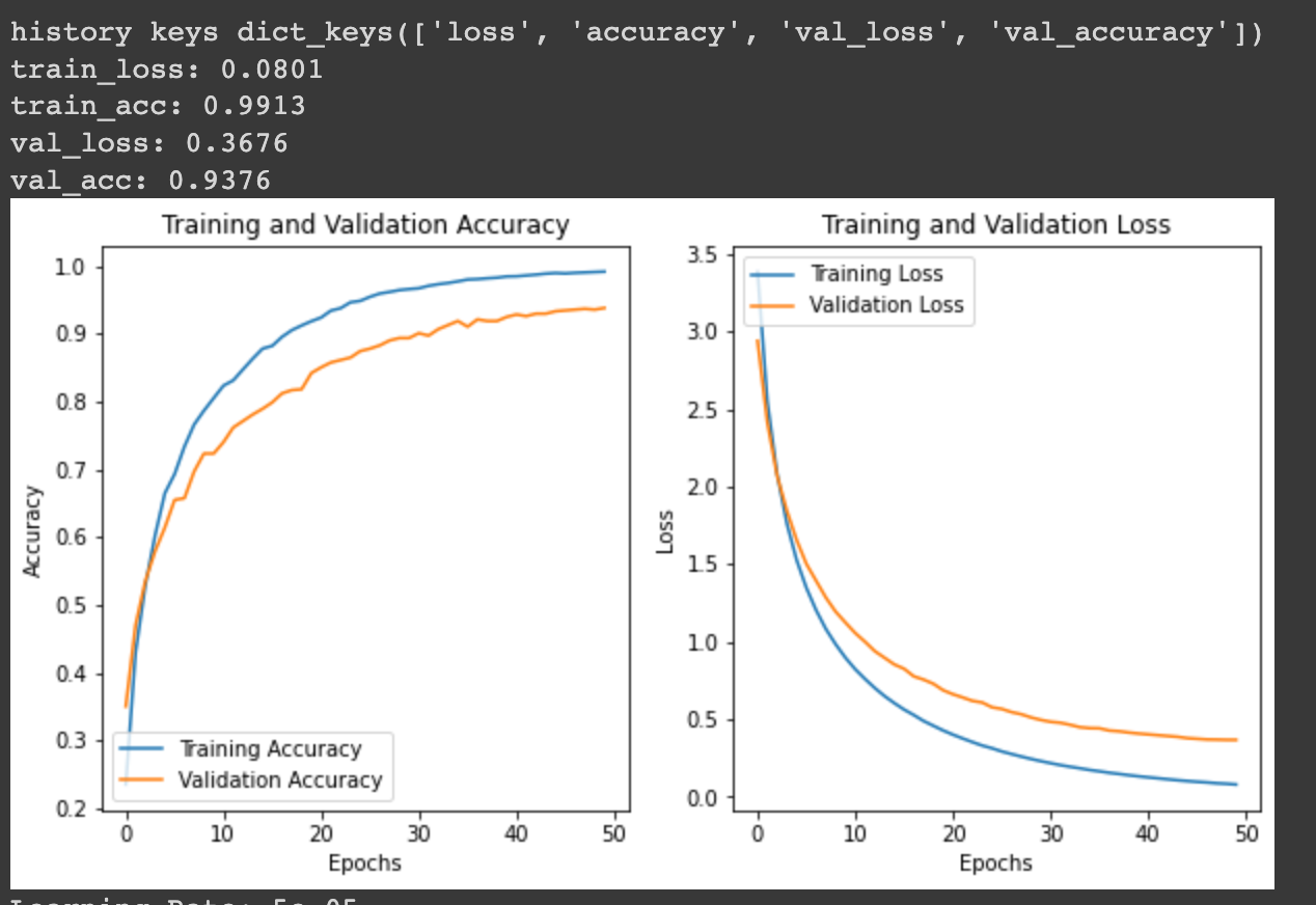
print("Training Ends!\nElapsed Time:", End_Time) 

The most optimized with an experimental approach (Manually adjusting learning rate and adding layers) is as follows.

Early-Stopping callback will reduce my wasting time by stopping training if enough training has been done.

Prediction

import PIL
import os
from random import randint

# Path where to pick random img from my Test Directory. 
path_test = "/content/my_data/traffic_Data/TEST/"
len_test = len(os.listdir(path_test)) - 1
rand_num = randint(0,len_test)
pick_any_img = os.listdir(path_test)[rand_num]

# Preprocess for picked img. 
img = keras.preprocessing.image.load_img(
    path_test + pick_any_img, target_size=(img_height, img_width)
)
img_array = keras.preprocessing.image.img_to_array(img)
img_array = tf.expand_dims(img_array, 0) 

# Run built model to predict a score after a softmax
predictions = model.predict(img_array)
score = tf.nn.softmax(predictions[0])

# Display picked img 
display(img.resize((120,120)))

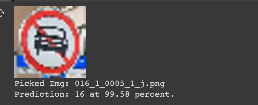
print("Picked Img: {}".format(pick_any_img))
print("Prediction: {} at {:.2f} percent.".format(class_names[np.argmax(score)], 100 * np.max(score)))

model.predict(img_array) predicts a lable with a given image. The prediction for label 16 is 99.58 percent in my case. But as the dataset has very limetted or my model has not yet been so much pricise, sometime it returns large error at some point.

Conclusion

Enough is enough. Although, the model isn't so perfect to be used practically, this projects guided me how build basic CNN model !