[TIL_Carrotww] 27 - 22/10/11

📝Carrotww의 코딩 기록장

🧲 Kaggle Data 활용해보기

🔍 Salary - 연차에 따른 연봉 변화도
연차가 입력으로 들어가고 연봉이 출력으로 나오는 단일 선형 형태로 쉬운편에 속한다.
난 처음해봐서 어렵다...

🔍

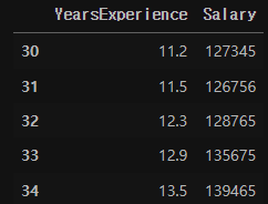
import os
os.environ['KAGGLE_USERNAME'] = 'carrotww' # username
os.environ['KAGGLE_KEY'] = 
# kaggle_key는 본인 키를 붙여서 항상 사용하면 된다.

!kaggle datasets download -d rsadiq/salary
# 해당 데이터를 다운로드 한 후
!unzip salary.zi
# 압축을 풀어준다.

from tensorflow.keras.models import Sequential
from tensorflow.keras.layers import Dense
from tensorflow.keras.optimizers import Adam, SGD
import numpy as np
import pandas as pd
import matplotlib.pyplot as plt 
import seaborn as sns
from sklearn.model_selection import train_test_split

df = pd.read_csv('Salary.csv')
# 압축을 풀어준 파일을 pandas의 read_csv 함수로 
# 읽어서 df에 저장

df.tail(5)

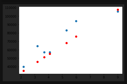
x_data = np.array(df['YearsExperience'], dtype=np.float32)
# x data는 연차를 넣어 numpy array로 변경해 주며
# 머신러닝 학습시에는 대부분 float 자료형으로 사용
y_data = np.array(df['Salary'], dtype=np.float32)

x_data = x_data.reshape((-1, 1))
y_data = y_data.reshape((-1, 1))
# 데이터가 한 개 이므로 1 을 넣어준다.

print(x_data.shape)
print(y_data.shape)

x_train, x_val, y_train, y_val = train_test_split(x_data, y_data, test_size=0.2, random_state=2021)
# test set을 20%로 나누어 준다

print(x_train.shape, x_val.shape)
print(y_train.shape, y_val.shape)

model = Sequential([
  Dense(1)
])
# 해당 모델을 선형 회귀로 만들어줌

model.compile(loss='mean_squared_error', optimizer=SGD(lr=0.01))
# optimizer는 SGD learning rate 는 0.01 로 사용
# optimizer는 아담으로도 변경 가능

model.fit(
    x_train,
    y_train,
    validation_data=(x_val, y_val), # 검증 데이터를 넣어주면 한 epoch이 끝날때마다 자동으로 검증
    epochs=100 # epochs 복수형으로
    # fit을 하여 학습을 시켜줌

y_pred = model.predict(x_val)
# x_val 데이터를 예측하여 y_pred에 넣어줌
plt.scatter(x_val, y_val)
plt.scatter(x_val, y_pred, color='r')
# 예측한 값을 red 로 그려줌
plt.show()

🧲 논리 회귀 (Logistic regression)

🔍 논리 회귀란 ?
쉽게 말해 선형 회귀로 풀 수 없는 문제를 풀기 위해 logistic(sigmoid) function 을 사용한다.

🔍 만약 출력 수치가 정해진 값이 궁금하다면?
가령 통과, 실패 같은 True False 와 같은 값은 선형회귀 그래프로 표현하기 어렵다.
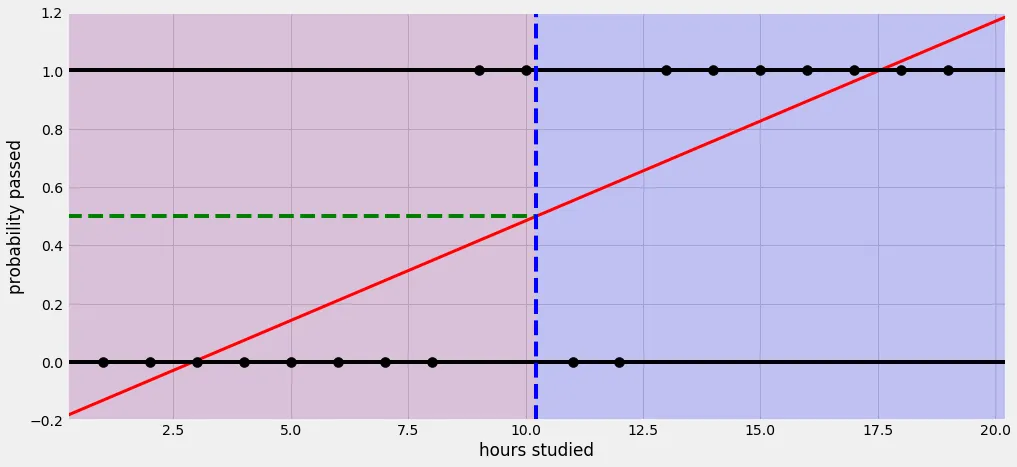
예를 들어 학점이 아닌 pass/fail 과목이 있을 때 몇 시간을 공부해야 pass가 나오는지 궁금하다. 10시간을 공부해야 pass가 나온다면 5, 6, 7시간을 공부했을때는 무조건 fail인가?

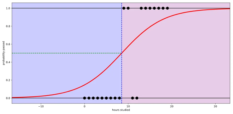
만약 그렇다면 위와 같은 그래프로 나올 것이다. 하지만 logistic(sigmoid) function을 사용한다면 아래와 같은 그래프로 나오게 된다.

해당 그래프에서는 확률에 따른 pass/fail 여부를 50%로 정하였다.

🔍 선형 회귀에서의 가설은 H(x) = Wx + b 식이며 논리 회귀에서는 시그모이드 함수에 선형회귀 수식을 넣은 것.
쉽게 결과값이 0 ~ 1이 나오게 하고 싶어서 나온 것이 논리 회귀 이다. 수학적인 부분 보다는 이해가 중요하기 때문에 수식은 pass..ㅎㅎ

🧲 Crossentropy 란

🔍 논리 회귀 그래프를 예측한 그래프로 만들기 위해서 도와주는 손실 함수 이다.