해당 문서는 Coursera 강의 Bayesian Statistics: Techniques and Models
를 보고 공부한 것을 정리한 노트입니다.
1. Monte Carlo Estimation
확률분포의 기대치를 구하려면 우리가 익히 아는 적분식 을 사용해야 한다.
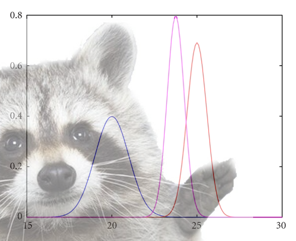
예를 들어 감마 분포를 따르는 확률변수 를 가정해 보자.
감마분포의 기대치는 감마분포의 pdf과 확률변수를 곱한 것을 적분하여 얻을 수 있다.
물론 항상 적분해서 구하지는 않고 보통 공식을 이용한다.
이렇게 공식이 있는 확률분포라면 확률변수의 기대치를 구하는 데 큰 문제가 없지만, 이전 포스트의 마지막에 있던 사후확률분포 같은 non-conjugate 확률분포에 관해서는 직접 적분을 하여 계산해야 한다.
가 분모에 들어가는 등 딱 봐도 적분하기 어렵게 생겼다...
Monte Carlo Integration
Expecation
아까 가정했던 확률변수 의 모분포 에서 뽑은 i번째 random sample을 라고 하자.
여기서 m은 충분히 큰 수라고 두고, 추출된 random sample을 더해서 평균을 낸다면 가 될 것이다. 그렇다면 큰 수의 법칙에 따라서 이 표본평균 은 모평균 에 확률수렴할 것이다.
따라서 이렇게 수식으로 표현할 수 있다.
이것이 Monte Carlo Integration의 기본 알고리즘이다.
Variance
같은 방법으로 sample variance로 모분산을 추정할수도 있다.
이때 m은 충분히 큰 수라고 정의했으므로 표본분산을 구할 때 m-1로 나눌 필요는 없다.
function of theta
위와 같은 방식으로, 에 대한 function에 대해서도 Monte Carlo Integration을 적용할 수 있다.
2. Python 코드 실습
import numpy as np
from scipy.stats import gamma
import matplotlib.pyplot as plt

# gamma(2,2)의 평균은 1입니다.
mean_true = gamma(a=2, scale=1/2).mean()

# gamma(2,2)에서 random samling으로 m개의 값을 추출해 평균을 냅니다.
temp = []
for i in range(0,8):
    m = int(float(f'1e+{i}'))
    theta_bar = np.sum(gamma.rvs(a=2, loc=0, scale=1/2, size=m, random_state=42)) * 1/m
    temp.append(theta_bar)

# sampling된 값(m)이 클수록 true값에 근사합니다.
plt.plot(temp, label='sample mean')
plt.hlines(y = theta_true, xmin=0, xmax=7, colors = 'r', label='true mean')
plt.xlabel('1e+x')
plt.legend()
plt.title('Monte Carlo Integration for theta ~ Gamma(2,2)')
plt.show()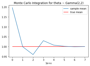
내용에 대한 질문, 잘못된 부분에 대한 지적 모두 환영합니다!