2023-1-OC-AI-Study-Week3

glob.glob / pd.concat()

여러 csv 불러와서 하나의 dataframe 만들기.

from glob import glob
warnings.filterwarnings('ignore') # 경고 메세지 무시

file_list = glob('03_EDA_실습데이터/*.csv')

ori_df = pd.DataFrame()

for i in range(len(file_list)):
    ori_df = pd.concat([ori_df, pd.read_csv(file_list[i])], axis=0)

str.contains(, na=False)

특정 열 조건 만족하는 행만 추출

concat_df['ismaposb'] = 
concat_df['지점명'].str.contains('마포|서강|홍대|상암|서교|합정',na=False) 
& concat_df['상호명'].str.contains('스타벅스',na=False)

concat_df = concat_df[concat_df['ismaposb'] == True]

missingno

결측치 시각화.

msno.matrix(df.iloc[:, :], color=(0.1, 0.6, 0.8))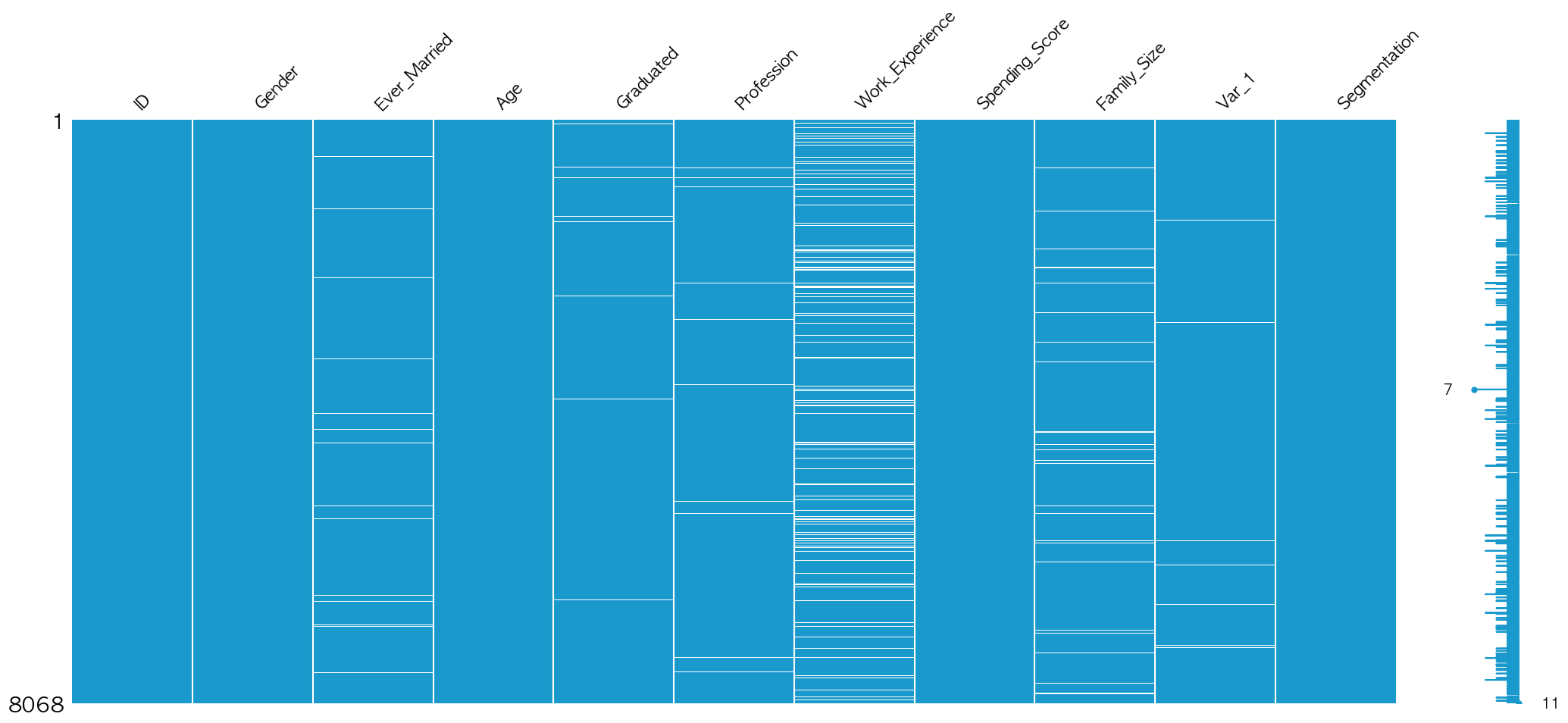

msno.bar(df.iloc[:, :])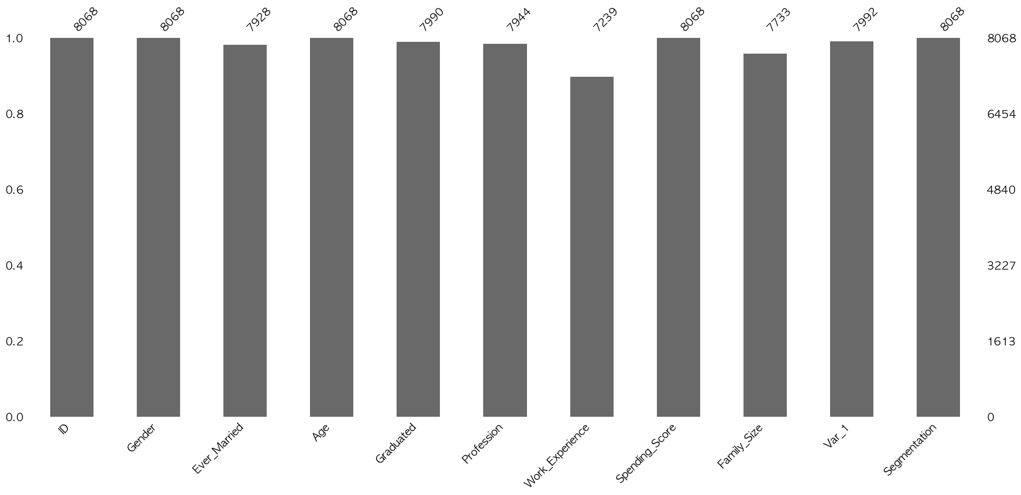

sns.countplot(x,data)

plt.figure(figsize=(20, 8))
plt.subplot(5,2,1)
sns.countplot(x='Gender', data=df)
plt.subplot(5,2,2)
sns.countplot(x='Ever_Married', data=df)
plt.subplot(5,2,3)
sns.countplot(x='Graduated', data=df)
plt.subplot(5,2,4)
plt.xticks(rotation=45)
sns.countplot(x='Profession', data=df)
plt.subplot(5,2,5)
sns.countplot(x='Spending_Score', data=df)
plt.subplot(5,2,6)
sns.countplot(x='Var_1', data=df)
plt.subplot(5,2,7)
sns.countplot(x='Segmentation', data=df)
plt.subplot(5,2,8)
sns.countplot(x='Work_Experience', data=df)
plt.subplot(5,2,9)
sns.countplot(x='Family_Size', data=df)
plt.subplot(5,2,10)
sns.histplot(data=df, x='Age', bins=16, kde=True)
plt.show()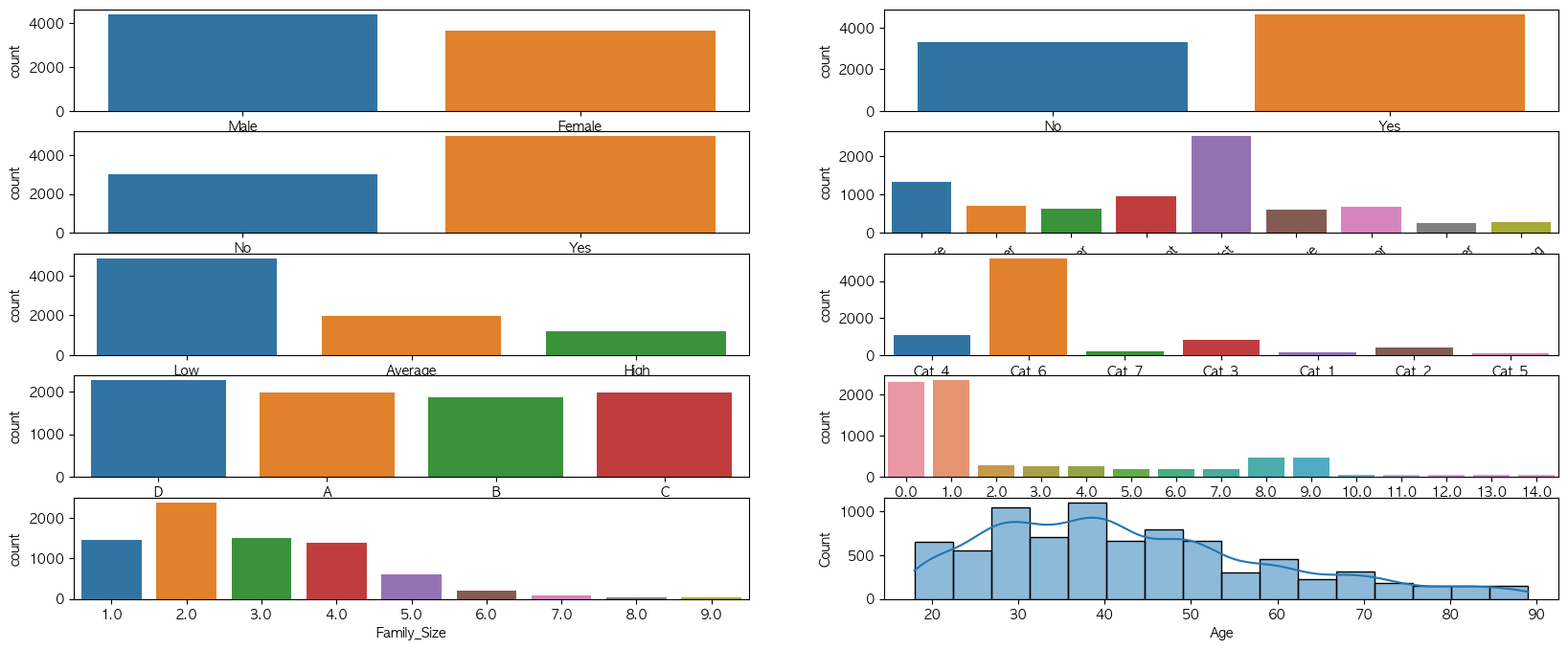

sns.heatmap

seaborn.heatmap(data, *, vmin=None, vmax=None, cmap=None, center=None,
robust=False, annot=None, fmt='.2g', annot_kws=None, linewidths=0, linecolor='white', 
cbar=True, cbar_kws=None, cbar_ax=None, square=False, 
xticklabels='auto', yticklabels='auto', mask=None, ax=None, **kwargs)

• heatmap 그리려면 df.corr()가 필요.
• non-numeric data를 numeric-data로 변환해준다.

# 예시
profession_ratio = {
    'Artist': 0.33,
    'Healthcare': 0.16,
    'Entertainment': 0.12,
    'Doctor': 0.09,
    'Engineer': 0.09,
    'Executive': 0.08,
    'Lawyer': 0.08,
    'Marketing': 0.03,
    'Homemaker': 0.03
}
for i in profession_ratio:
    for j in range(len(df)):
        df.loc[df['Profession']==i,'Profession'] = profession_ratio[i]
df['Profession'] = pd.to_numeric(df['Profession'])

• df.corr(method='pearson', min_periods=1)
  method : {pearson / kendall / spearman}
  min_periods : 유효한 결과를 얻기위한 최소 값의 수 입니다. (피어슨, 스피어먼만 사용가능)
• df.corrwith(other, axis=0, drop=False, method='pearson')
  other : 동일한 이름의 행/열을 비교할 다른 객체입니다.
  axis : {0 : index / 1 : columns} 비교할 축 입니다. 기본적으로 0으로 인덱스끼리 비교합니다.
  drop : 동일한 이름의 행/열이 없을경우 NaN을 출력하는데, 이를 출력하지 않을지 여부입니다.
  method : {pearson / kendall / spearman}

import numpy as np
mask=np.zeros_like(df.corr(),)
mask[np.triu_indices_from(mask)]=True
sns.heatmap(round(df.corr(),2), annot=True,mask=mask)

---

참고

• https://velog.io/@songjeongwoo/Seaborn%EC%9D%84-%EC%9D%B4%EC%9A%A9%ED%95%9C-%EC%8B%9C%EA%B0%81%ED%99%94
• https://wikidocs.net/45798 (한글 깨짐)
• https://hong-yp-ml-records.tistory.com/14
• https://velog.io/@rlarudans/%ED%95%9C-%EB%B2%88%EC%97%90-Graph-%EC%97%AC%EB%9F%AC-%EA%B0%9C-%EA%B0%99%EC%9D%B4-%EC%B6%9C%EB%A0%A5%ED%95%98%EA%B8%B0
• https://seaborn.pydata.org/generated/seaborn.heatmap.html
• https://wikidocs.net/157461