[논문 리뷰] Precursor-of-Anomaly Detection for Irregular Time Series

‍이진혁[ 대학원석·박사통합과정재학 / 산업경영공학과 ]·2026년 7월 28일

Paper Seminar

목록 보기

19/20

이 논문은 현재 시계열 구간의 이상 여부를 판별하는 anomaly detection과, 현재 구간을 이용해 다음 미래 구간의 이상 발생 여부를 예측하는 Precursor-of-Anomaly(PoA) detection을 함께 정의함.
제안 모델 PAD는 두 개의 Neural Controlled Differential Equation(NCDE), multi-task learning, knowledge distillation, self-supervised anomaly augmentation을 결합함

1. 연구 배경

일반적인 시계열 이상탐지는 현재 또는 이미 관측된 시계열에서 정상 패턴과 다른 구간을 찾는 문제다. 논문에서는 이를 다음 질문으로 표현함

현재 입력 시계열 구간에 이상 관측치가 포함되어 있는가?

이 논문은 여기에 미래 구간에 관한 문제를 추가함

현재까지 관측된 시계열을 이용해, 다음 미래 구간에 이상 관측치가 포함될지를 예측할 수 있는가?

저자들은 두 번째 문제를 Precursor-of-Anomaly detection, 줄여서 PoA detection이라고 정의한다. 이때 precursor는 미래의 이상 발생과 연결되는 현재의 패턴 또는 징후를 의미함.

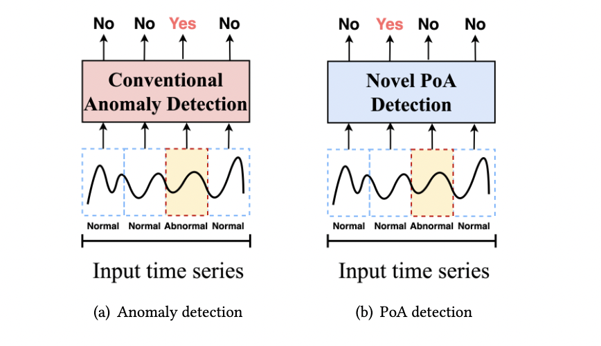
Anomaly detection은 현재 구간을 분류하고, PoA detection은 현재 구간을 입력으로 다음 미래 구간의 이상 포함 여부를 예측함.

2. 문제 정의

2.1 다변량 시계열

논문은 길이 $T$ 인 다변량 시계열을 다음과 같이 정의함

\mathbf{x}_{0:T} = \{\mathbf{x}_0,\mathbf{x}_1,\ldots,\mathbf{x}_T\}, \qquad \mathbf{x}_t\in\mathbb{R}^{N}

여기서 $N$ 은 변수의 개수

Regular time series에서는 연속된 관측 시점 사이의 간격이 일정한 반면 irregular time series에서는 관측 간격이 일정하지 않음

2.2 윈도우 구성

전체 시계열은 크기 $b$ 인 non-overlapping window로 나뉜다.

w_i = [\mathbf{x}_{t_0^i},\mathbf{x}_{t_1^i},\ldots,\mathbf{x}_{t_b^i}]

각 윈도우는 anomaly detection 또는 PoA detection의 입력 단위가 된다.

2.3 두 개의 분류 과제

현재 입력 윈도우를 $w_i$ , 바로 다음 윈도우를 $w_{i+1}$ 이라고 하면 논문의 두 과제는 다음과 같다.

Anomaly detection: $w_i$ 에 이상 관측치가 포함되어 있는지를 이진 분류한다.
PoA detection: $w_i$ 만 입력받아 $w_{i+1}$ 에 이상 관측치가 포함될지를 이진 분류한다.

현재 입력 구간                     다음 미래 구간
┌──────────────┐                  ┌──────────────┐
│     w_i      │                  │   w_{i+1}    │
└──────────────┘                  └──────────────┘

Anomaly detection: w_i가 정상인가, 이상인가?
PoA detection:     w_{i+1}에 이상이 포함될 것인가?

PAD의 PoA 출력은 미래 값을 직접 생성하는 forecasting 결과가 아니라, 다음 미래 윈도우의 이상 포함 여부에 대한 binary classification 결과다.

3. 배경 개념

3.1 Neural Controlled Differential Equation

논문은 irregular time series를 처리하기 위해 NCDE를 사용한다.

이산 관측이

\{(\mathbf{x}_i,t_i)\}_{i=0}^{N}

로 주어지면, interpolation을 통해 연속시간 경로 $X(t)$ 를 만든다. 논문은 일반적인 NCDE 설정에서 사용되는 natural cubic spline을 설명한다.

NCDE의 hidden state는 다음과 같이 정의된다.

\mathbf{z}(T) = \mathbf{z}(0) + \int_0^T f(\mathbf{z}(t);\theta_f)\,dX(t)

이를 시간에 대한 적분 형태로 쓰면 다음과 같다.

\mathbf{z}(T) = \mathbf{z}(0) + \int_0^T f(\mathbf{z}(t);\theta_f) \frac{dX(t)}{dt}\,dt

NCDE는 보간된 입력 경로 $X(t)$ 에 의해 hidden state가 연속적으로 변화하는 구조다. 논문에서는 이를 RNN의 continuous-time analogue로 설명한다.

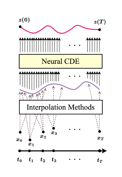
불규칙하게 관측된 이산 시계열을 interpolation한 뒤 Neural CDE가 hidden state를 계산하는 구조

3.2 Multi-task learning

Multi-task learning은 여러 과제를 독립적으로 학습하지 않고, 일부 파라미터 또는 표현을 공유하면서 함께 학습하는 방식이다.

논문은 다음 세 가지 parameter sharing 유형을 소개한다.

Hard parameter sharing
Soft parameter sharing
Task-specific parameter sharing

PAD는 anomaly task와 PoA task가 각자의 파라미터를 가지면서 일부 파라미터를 공유하는 task-specific parameter sharing 구조를 사용한다.

3.3 Knowledge distillation

Knowledge distillation은 teacher model의 출력을 student model의 학습 신호로 사용하는 방법이다.

PAD에서는 다음 미래 윈도우를 직접 입력받은 anomaly NCDE가 teacher 역할을 하고, 현재 윈도우만 입력받는 PoA NCDE가 student 역할을 한다.

4. PAD 전체 구조

PAD는 (Precursor of) Anomaly Detection의 약자다. 모델은 anomaly detection용 NCDE와 PoA detection용 NCDE로 구성된다.

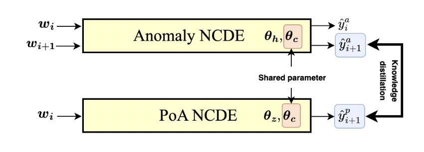
PAD 전체 구조. 위쪽 anomaly NCDE, 아래쪽 PoA NCDE, 공유 파라미터 $\theta_c$ , anomaly branch에서 PoA branch로 전달되는 knowledge distillation 관계가 표시되어 있다.

논문이 제시한 전체 학습 흐름은 다음과 같다.

정상 training sequence에 augmentation을 적용해 인공 이상 구간을 만든다.
Anomaly NCDE와 PoA NCDE가 각각 hidden representation을 생성한다.
Anomaly NCDE는 현재 윈도우 $w_i$ 와 다음 윈도우 $w_{i+1}$ 을 학습 과정에서 입력받는다.
Anomaly detection과 PoA detection을 위한 두 개의 output layer를 둔다.
두 NCDE는 공유 파라미터 $\theta_c$ 를 통해 multi-task learning을 수행한다.
Anomaly NCDE가 $w_{i+1}$ 에 대해 생성한 출력을 PoA NCDE의 distillation target으로 사용한다.

5. Dual co-evolving NCDE

5.1 두 hidden state

PAD는 anomaly detection용 hidden state $h(t)$ 와 PoA detection용 hidden state $z(t)$ 를 각각 계산한다.

h(T) = h(0) + \int_0^T f\big(h(t);\theta_f,\theta_c\big) \frac{dX(t)}{dt}\,dt

z(T) = z(0) + \int_0^T g\big(z(t);\theta_g,\theta_c\big) \frac{dX(t)}{dt}\,dt

각 파라미터의 역할은 다음과 같다.

$\theta_f$ : anomaly NCDE에만 사용되는 task-specific parameter
$\theta_g$ : PoA NCDE에만 사용되는 task-specific parameter
$\theta_c$ : 두 NCDE가 함께 사용하는 shared parameter

5.2 Vector field의 구성

논문에서 $f$ 와 $g$ 는 task-specific network와 shared network의 출력을 합하는 형태로 정의된다.

f(h(t);\theta_f,\theta_c) = f_{\theta_f}(h(t))+f_{\theta_c}(h(t))

g(z(t);\theta_g,\theta_c) = g_{\theta_g}(z(t))+g_{\theta_c}(z(t))

각 network는 fully connected layer, ReLU, tanh를 사용한다. 두 NCDE는 $\theta_c$ 를 공동으로 갱신하므로 학습 과정에서 함께 변화한다.

5.3 출력층

Anomaly detection 출력은 다음과 같다.

\hat y_i^a = \sigma\left(\mathrm{FC}_{\theta_a}(h(T))\right)

PoA detection 출력은 다음과 같다.

\hat y_i^p = \sigma\left(\mathrm{FC}_{\theta_p}(z(T))\right)

$\sigma$ 는 sigmoid이며, 두 출력 모두 binary classification probability다.

5.4 동시 적분

구현에서는 두 hidden state를 하나의 augmented state로 구성하고 같은 ODE solver에서 함께 계산한다.

\frac{d}{dt} \begin{bmatrix} h(t)\\ z(t) \end{bmatrix} = \begin{bmatrix} f(h(t);\theta_f,\theta_c)\dfrac{dX(t)}{dt}\\ g(z(t);\theta_g,\theta_c)\dfrac{dX(t)}{dt} \end{bmatrix}

초기 hidden state는 $X(0)$ 을 fully connected layer에 통과시켜 만든다.

6. 학습 방법

6.1 Anomaly detection loss

현재 윈도우 $w_i$ 의 anomaly label을 $y_i$ 라고 하면 anomaly detection loss는 다음과 같다.

\mathcal{L}_a = \mathrm{CE}(\hat y_i^a,y_i)

6.2 Knowledge distillation loss

학습 과정에서 anomaly NCDE는 다음 윈도우 $w_{i+1}$ 을 직접 입력받아 anomaly probability $\hat y_{i+1}^a$ 를 생성한다.

PoA NCDE는 현재 윈도우 $w_i$ 만 입력받아 다음 구간에 관한 probability $\hat y_{i+1}^p$ 를 생성한다.

Knowledge distillation loss는 다음과 같다.

\mathcal{L}_{KD} = \mathrm{CE}(\hat y_{i+1}^a,\hat y_{i+1}^p)

즉, PoA NCDE는 미래 윈도우를 직접 본 anomaly NCDE의 출력을 모방하도록 학습된다.

6.3 파라미터별 업데이트

논문의 Algorithm 1은 파라미터를 다음과 같이 갱신한다.

$\theta_f$ : $\mathcal{L}_a$ 로 학습
$\theta_g$ : $\mathcal{L}_{KD}$ 로 학습
$\theta_c$ : $\mathcal{L}_a$ 와 $\mathcal{L}_{KD}$ 를 함께 사용해 학습
Output layer와 초기 상태 관련 파라미터도 각 loss에 따라 함께 갱신

학습에는 adjoint sensitivity method가 사용된다. 논문은 두 NCDE를 사용하기 때문에 필요한 메모리를 $O(2T+H_f+H_g)$ 로 설명한다.

7. Self-supervised anomaly augmentation

Anomaly detection benchmark는 일반적으로 training set에는 정상 데이터만 제공하고 test set에 anomaly label을 제공한다. PAD는 정상 training sequence에 인공 이상을 삽입해 학습 데이터를 구성한다.

논문에 제시된 augmentation 절차는 다음과 같다.

데이터셋의 anomaly ratio를 $\gamma=L/T$ 로 유지한다.
인공 이상 구간의 시작 위치를 무작위로 선택한다.
이상 구간 길이를 100에서 500 사이에서 무작위로 선택한다.
Training sequence의 다른 위치에서 구간을 무작위로 선택한다.
선택한 구간을 목표 위치에 copy-and-paste한다.
Augmentation은 원본 long sequence에 먼저 적용한 뒤 윈도우로 분할한다.

이 방법은 정상 시계열 내부의 한 구간을 다른 위치로 이동시켜 문맥이 달라진 패턴을 인공 anomaly로 사용한다.

8. 실험 설정

8.1 데이터셋

데이터셋	설명	변수 수	테스트 이상 비율
MSL	NASA Mars Science Laboratory 장비 health-check telemetry	55	약 10.72%
SWaT	수처리 공정 testbed의 정상 및 공격 시나리오 데이터	51	약 11.98%
WADI	물 분배 공정 testbed의 정상 및 공격 시나리오 데이터	123	약 5.99%

8.2 주요 설정

데이터셋	Epoch	Learning rate	Weight decay	$\theta_f/\theta_g/\theta_c$ hidden size	입력 window length	PoA prediction length
MSL	300	$10^{-2}$	$10^{-4}$	256 / 512 / 256	30	10
SWaT	300	$10^{-2}$	$10^{-4}$	128 / 64 / 64	60	20
WADI	300	$10^{-2}$	$10^{-5}$	128 / 128 / 256	100	30

8.3 Regular 및 irregular setting

Regular setting: 원래 데이터의 관측 시점을 그대로 사용한다.
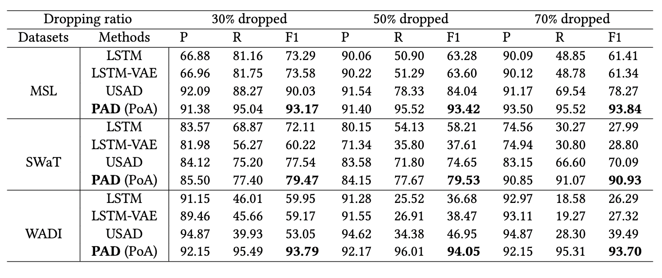
Irregular setting: 각 sequence의 관측치를 무작위로 30%, 50%, 70% 제거한다.

8.4 비교 모델

논문은 다음 계열의 모델들과 비교한다.

Classical: OCSVM, Isolation Forest
Clustering-based: Deep-SVDD, ITAD, THOC
Density-estimation-based: LOF, DAGMM, MMPCACD
Reconstruction 또는 prediction 기반: VAR, LSTM, CL-MPPCA, LSTM-VAE, BeatGAN, OmniAnomaly, USAD, InterFusion, Anomaly Transformer

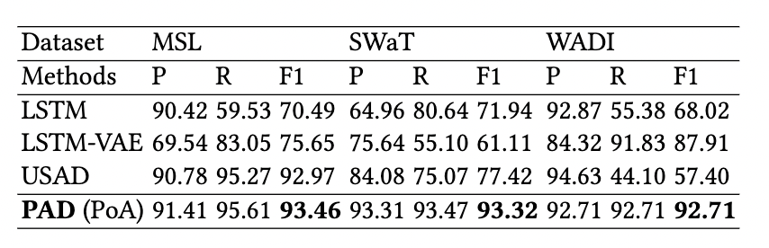
PoA detection 실험에서는 LSTM, LSTM-VAE, USAD와 비교한다.

평가지표는 Precision, Recall, F1-score다.

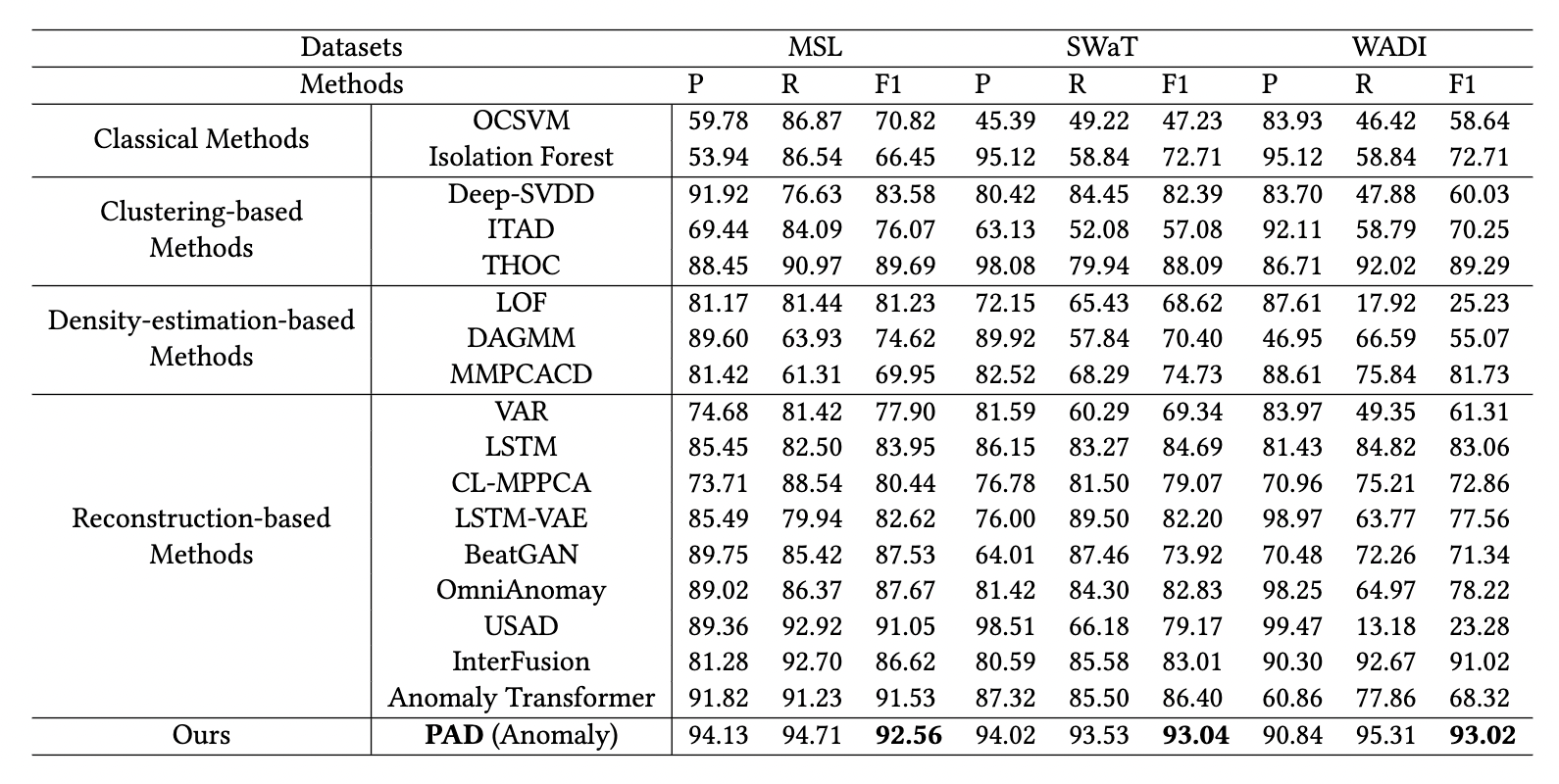
9. Anomaly detection 결과

9.1 Regular time series

Table 1에 보고된 PAD의 결과는 다음과 같다.

9.2 Irregular time series

관측치 제거 비율에 따른 PAD anomaly F1-score는 다음과 같다.

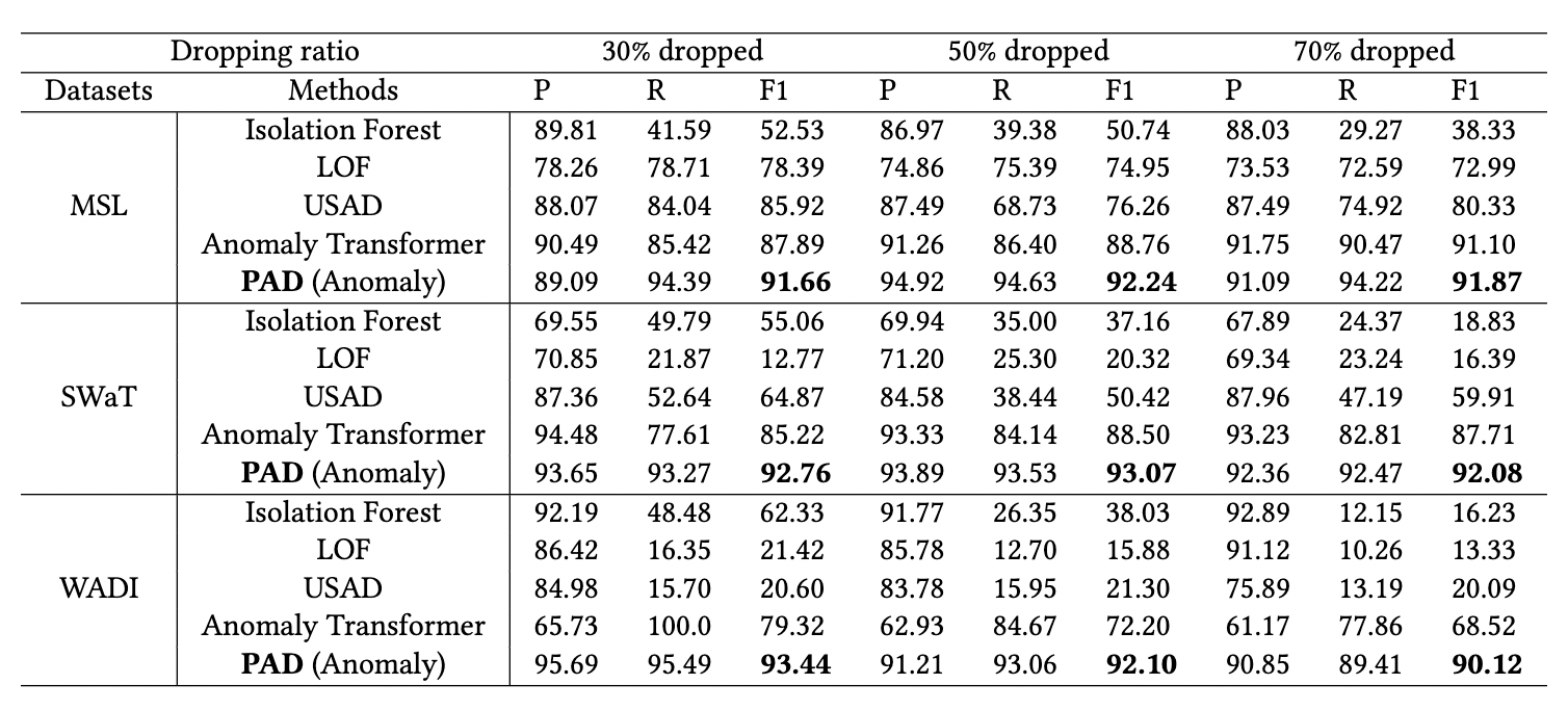
논문은 NCDE가 보간된 continuous path $X(t)$ 를 통해 hidden representation을 계산하기 때문에 irregular setting에서도 성능을 유지한다고 설명한다.

10. PoA detection 결과

10.1 Regular time series

Table 3의 F1-score는 다음과 같다.

10.2 Irregular time series

PAD PoA의 F1-score는 다음과 같다.

10.3 결과 시각화

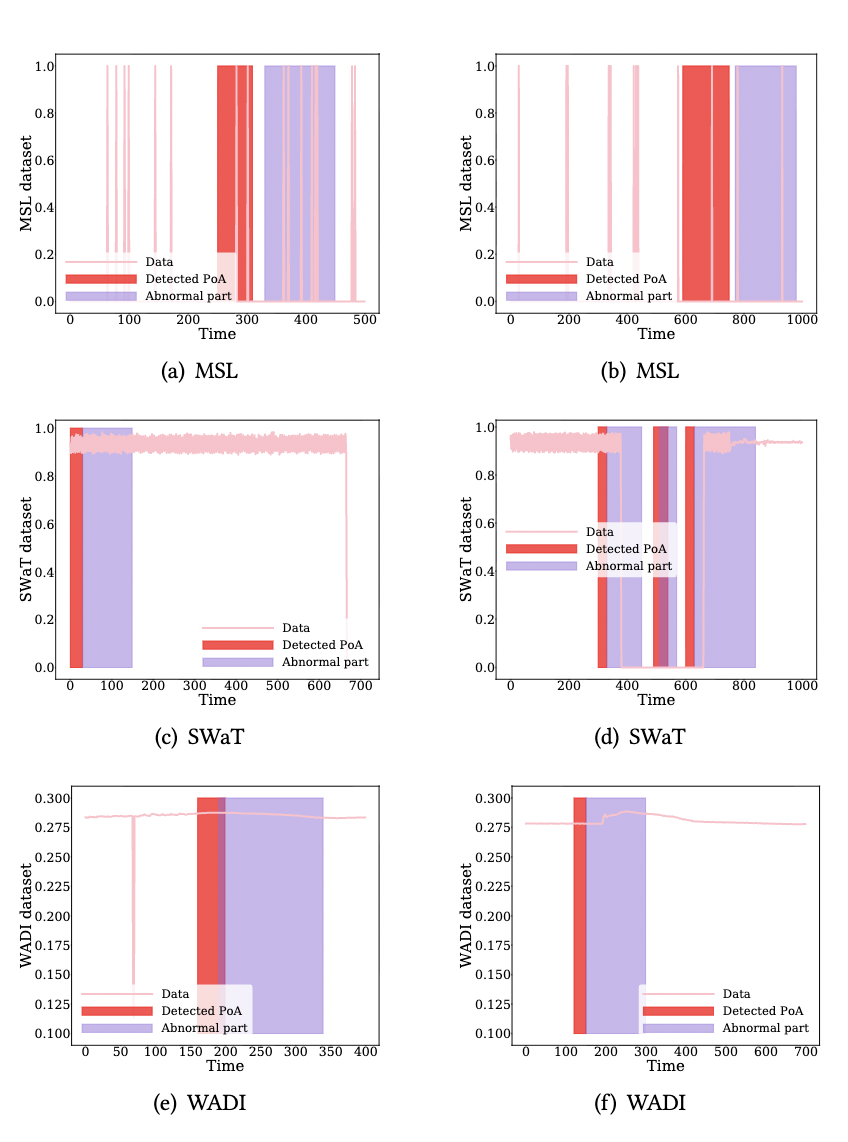
Figure 5는 MSL, SWaT, WADI의 일부 구간을 시각화한다.

보라색 영역: 실제 anomaly 구간
빨간색 영역: PAD가 탐지한 PoA 구간
선 그래프: 데이터 값

논문은 여러 예시에서 빨간색 PoA 구간이 실제 anomaly 구간보다 앞에 나타나는 결과를 제시한다.

11. Ablation study

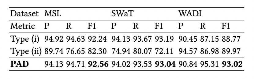
논문은 anomaly detection task와 PoA detection task를 함께 학습하는 multi-task setting을 확인하기 위해 두 종류의 ablation model을 구성한다. 표에서는 이를 Type (i), Type (ii)로 표시한다.

11.1 Anomaly detection ablation

11.2 PoA detection ablation

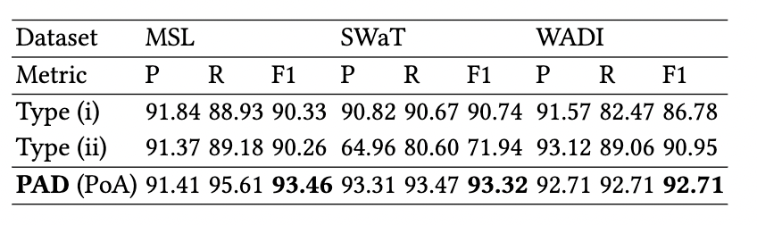
논문은 한 task를 제거한 경우 anomaly detection 또는 PoA detection 성능이 감소하는 결과를 multi-task learning의 효과로 설명한다.

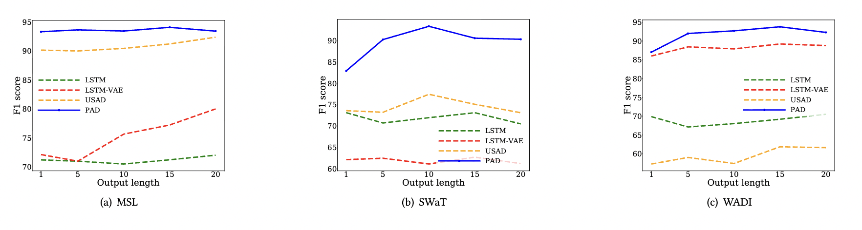
12. Output sequence length sensitivity

입력 길이는 30으로 고정하고 PoA output length를 다음과 같이 변경한다.

\{1,5,10,15,20\}

비교 모델은 LSTM, LSTM-VAE, USAD이며, Figure 4는 MSL, SWaT, WADI에서 output length에 따른 F1-score 변화를 보여준다.

13. 논문의 결론과 향후 계획

논문은 PoA detection을 미래 anomaly를 예측하는 과제로 정의하고, anomaly detection과 PoA detection을 하나의 dual-NCDE framework에서 함께 학습한다.

제안 방법을 구성하는 요소는 다음과 같다.

Irregular time series를 처리하는 NCDE
Anomaly NCDE와 PoA NCDE로 구성된 dual co-evolving architecture
두 task 사이의 task-specific parameter sharing
Anomaly NCDE를 teacher로 사용하는 knowledge distillation
정상 training sequence에서 인공 anomaly를 생성하는 self-supervised augmentation

저자들은 향후 연구로 unsupervised precursor-of-anomaly detection을 제시한다. 현재 방법의 time-series augmentation이 별도의 preprocessing 단계를 필요로 하기 때문이다.

‍이진혁[ 대학원석·박사통합과정재학 / 산업경영공학과 ]

Researcher

이전 포스트

[논문 리뷰] Adaptive Turbofan Engine Health Assessment for Multi-component Performance Degradation Coupling Scenarios: A Spatiotemporal Attention Graph Convolutional Network Approach

다음 포스트