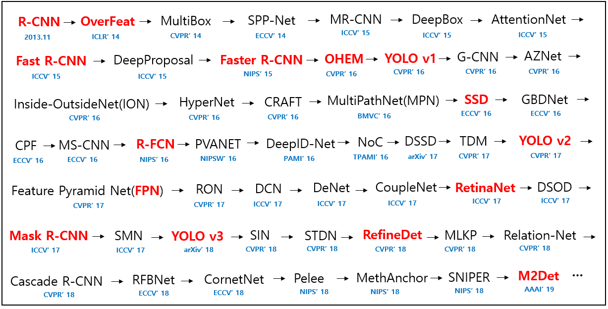
오늘 리뷰할 논문은 R-CNN과 동시대에 나온 object detection 모델이며 ILSVRC 2013 localization task의 우승자인 OverFeat이다. R-CNN 논문에서 OverFeat와 성능을 비교한 부분이 있어 호기심이 생겨 읽게 되었다.
아래 포스트를 먼저 읽으면 도움이 될 것이다.
- [Deeplearning] OverFeat: Integrated Recognition, Localization and Detection using Convolutional Networks
- Overfeat 논문(Integrated Recognition, Localization and Detectionusing Convolutional Networks) 리뷰
- [논문리뷰] OverFeat
- OverFeat: Integrated Recognition, Localization and Detection using Convolutional Networks (번역)
Summary
논문은 multiscale, sliding window 방식의 접근을 통한 하나의 Convolutional Network으로 classification, localization, detection을 동시에 하는 것을 목적으로 한다. 또 localization과 detection을 위해 object boundary를 예측하고 (detection confidence를 향상시키도록 suppressed하는 대신) Bounding boxes를 accumulate하는 새로운 deep learning approach를 소개한다. 논문은 많은 localization predictions을 결합하는 것으로 background sample에 대한 복잡하고 시간 잡아먹는 학습 없이도 detection이 가능하다는 것을 제안한다. background 학습을 안 하는 건 network가 오직 positive classes에만 집중하게 해서 더 높은 정확도를 내기도 한다.
이 논문 모델의 classification architecture은 AlexNet과 비슷한데 network design과 inference step에서 발전이 있다.
이후에 더 설명하겠지만 training에선 모델이 1x1 크기의 output maps를 만들기 때문에 non-spatial이라고 하는데 inference step에선 spatial output을 만든다.
모델의 1-5층은 AlexNet과 유사해서 ReLU와 max pooling을 쓰지만 다음 세가지 측면에서 다르다. 1. contrast normalization을 사용하지 않고 2. pooling regions가 non-overlapping이고 3. 더 작은 stride 크기(4 대신 2)를 사용해서 1st, 2nd layer의 feature map이 더 크다.(더 큰 stride는 speed에서 유리하지만 accuracy가 낮다)
(참고로 논문은 classificatoin, localization, detection 각각에 대해 net을 만드는데 feature extractor인 layer 1-5는 공유하게 두고 마지막 FC layers들만 바꿔가며 각 task에 맞춘다.)
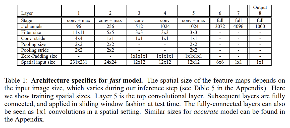
논문은 OverFeat라고 이름붙인 feature extractor를 고안한다. fast와 accurate 버전으로 모델 2개를 만들어 이후 실험한다.
또 multi-scale classification을 하는데 각 location에서 여러 scale로 network를 densely running해서 이미지 전체를 탐색한다. convnet에선 sliding window 방식이 효과적인데 voting을 위한 view가 더 많아서 robustness가 증가하기 때문이다. 임의의 크기의 이미지에 대한 convnet의 결과는 각 scale마다 C-dimensional vectors의 spatial map이다.
하지만 CNN의 total subsampling ratio이 2x3x2x3=36이 되는데, 다시 말해 36 pixel마다 하나의 classification vector를 만든다. 이런 coarse distribution은 10-view scheme에 비하면 성능이 떨어지는데 network windows가 이미지 내의 object와 잘 align되지 않기 때문이다. 이 문제를 해결하기 위해 모든 offset마다 마지막 subsampling operation을 실행해서 해당 층에서의 resolution loss를 없애 subsampling ratio를 2x3x2=12로 완화한다.
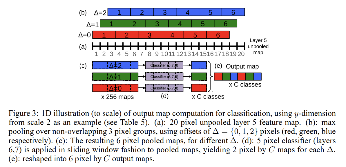
그럼 이런 resolution augmentation은 어떻게 하나? 6 scales의 input을 넣어 unpooled layer 5 maps of varying resolution를 도출한다. 이들은 다음의 순서에 따라 pool되고 classifier에게 전달된다.
- 하나의 이미지, 주어진 scale에서, unpooled layer 5 feature maps로 시작한다.
- 각 unpooled maps는 3x3 max pooling operation (non-overlapping regions)을 거치며 (∆x, ∆y) pixel offsets of {0, 1, 2}에 대해 3x3번 반복된다.
- 그럼으로써 서로 다른 (∆x, ∆y) 조합에 대해 3x3번 반복된 pooled feature maps의 집합을 얻게 된다.
- classifier (layers 6,7,8)은 5x5로 고정된 input 크기를 가지고 pooled maps 내의 각 location마다 C-dimensional output
vector를 생성한다. classifier는 pooled maps에 sliding-window 방식으로 적용되어 주어진 (∆x, ∆y) combination에 대해 C-dimensional output maps를 만든다. - 서로 다른 (∆x, ∆y) 조합에 대한 output maps가 하나의 3D output map으로(2 spatial dimensions x C classes) reshape된다.
이 작업은 subsampling 없이 classifier’s viewing window를 1 pixel씩 shift하고 다음 layer에서 skip-kernels를 사용하는 것으로 볼 수 있다.
위의 과정이 수평으로 뒤집힌 이미지에 대해서도 실행되고 최종 classification을 다음과 같은 과정으로 생산한다.
- 각 class, 각 scale과 flip에 대해 spatial max를 구하고
- 서로 다른 scale과 flip에서 나온 C-dimensional vectors 결과들을 average하고
- mean class vector에서 top-1/top-5 elment를 구한다
feature extraction layers (1-5)과 classifier layers (6-output)은 반대로 사용되는데, 연산량의 관점에서 이미지 위로 fixed-size feature extractor를 sliding해서 결과를 합치는 것보다 이 방법이 더 효율적이다. 하지만 classifier에선 다른 position과 scale에서 layer 5 feature maps 내의 fixed-size representation를 원하기 때문에 classifier은 fixed-size 5x5 input을 가지고 layer 5 maps에 exhaustively 적용된다.
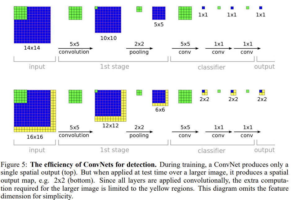
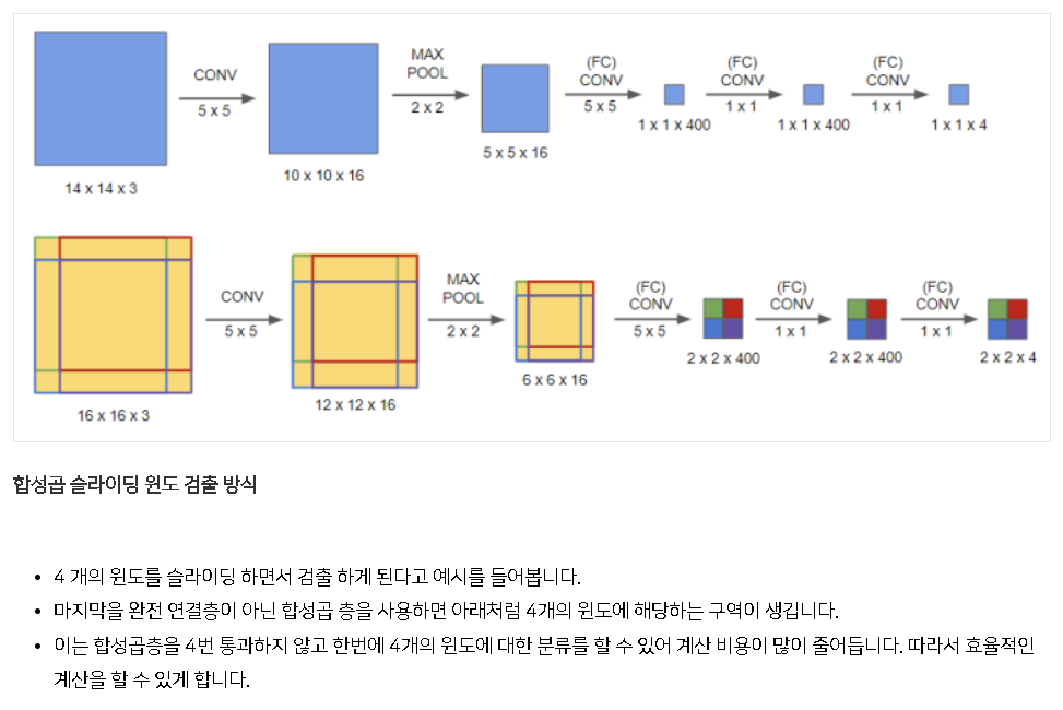
convnet가 sliding window보다 왜 효율적인지 살펴보자. convnet이 sliding fashion으로 적용됐을 때 overlapping region에 대해 연산을 공유한다. Fig 5를 보면 알 수 있듯 feature extraction layers를 통과하면 14x14가 1 spatial location을 도출하는데, (receptive field보다 더 큰, 예컨대) 16x16 영역을 계산하면 sliding window였다면 4번을 따로 계산해서 4개의 spatial location을 만들어야 했겠지만 convnet은 한 번만 계산해서 중복되는 연산을 줄일 수 있다.
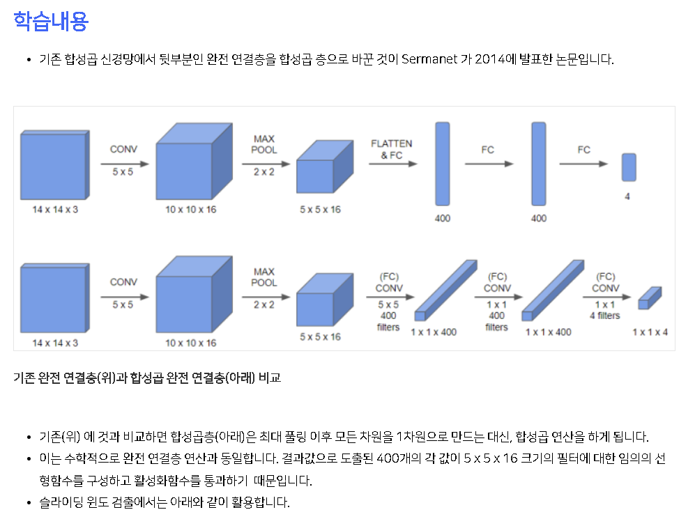
이때 architecture의 last layers(=classifier layers)은 fully connected layer인데 test time에선 1x1 convolution으로 바뀐다.
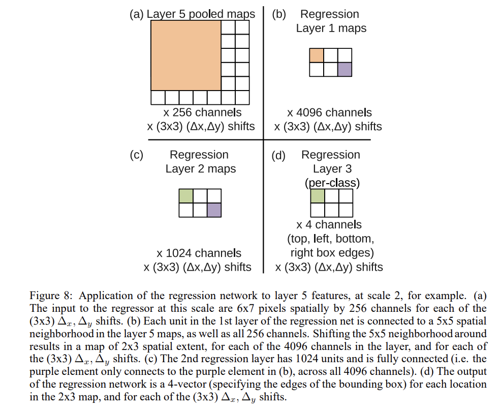
이제 classification은 됐고, localization은 어떻게 하나? 이렇게 classification-trained network를 만들고 나서 classifier layers를 regression network로 교체하는 것으로 각 spatial location과 scale에서 object bounding box를 예측한다. 그리고 각 location에서 regression predictions를 classification result를 결합한다.
classifier과 regressor network가 feature extraction layer를 공유하고 있기 때문에 classification network를 계산한 후 regression layers를 다시 계산하면 된다. 마지막 softmax layer은 c class에 대해 물체가 bounding box에 존재하는지 confidence score를 제공한다.
training의 경우 classification network에서 feature extraction layers (1-5)를 고정시키고 L2 loss를 이용해 regression network만 학습시킨다. 최종 regressor layer은 class-specific한데, 1000개의 다른 버전이 각 class에 할당된다는 의미다. 그리고 across-scale prediction combination를 위해 multi-scale manner로 regressor를 학습하는 게 중요하다.
논문은 (NMS 대신) regressor bounding boxes에 greedy merge strategy를 적용해 개별 prediction들을 합친다. 자세한 알고리즘은 아래와 같다.
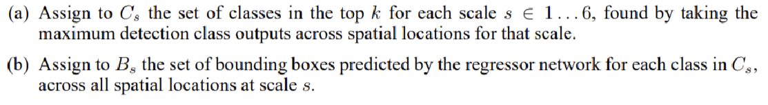
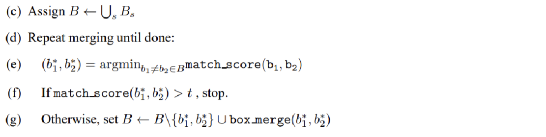
두 bounding box의 중심 간 거리와 box들의 intersection area의 합을 이용해 match_score을 계산한다. box_merge는 bounding box들의 좌표를 평균낸다.
최종 prediction은 maximum class scores를 가진 merged bounding boxes가 된다. 이 방법은 bounding box coherence를 rewarding함으로써 NMS보다 pure-classification model에서 오는 false positives에 더 robust하다.
detection은 spatial manner에서 classification training와 유사하다. 모델이 convolutional하기 때문에 모든 위치에서 weight가 공유되고 한 이미지에서 여러 location이 동시에 학습된다. localization task과 차이는 object가 존재하지 않을 때 background class를 예측해야한다는 점이다. negative example에 대해 이야기하는 부분도 있는데 생략하겠다.
Strengths
- 중복 연산을 피함으로써 sliding window 방식보다 Convnet이 효율적일 수 있다는 것을 설명했다.
- (사실 성능이 그렇게 뛰어난지는 잘 모르겠지만) NMS를 대체할 수 있는 새로운 알고리즘을 제안했다.
- 일종의 transfer learning처럼 feature extractor은 공유시키고 마지막 layer들만 교체하면서 각 task에 specialize되도록 fine-tuning한 방식이 인상적이었다.
논문의 설명이 너무 중구난방이라 architecture을 파악하기 어려웠다. 차라리 다른 리뷰어들의 포스트를 읽는 게 이해에 훨씬 더 도움이 됐다. (사실 아직도 잘 모르겠다)
또 Andrew Ng 교수님의 강의에도 OverFeat의 원리가 간략하게 설명되는데 보면 이해하기 좋을 것이다.
- https://www.boostcourse.org/ai218/lecture/410014?isDesc=false
또는
https://www.youtube.com/watch?v=XdsmlBGOK-k