MobileNets: Efficient Convolutional Neural Networks for Mobile Vision Applications

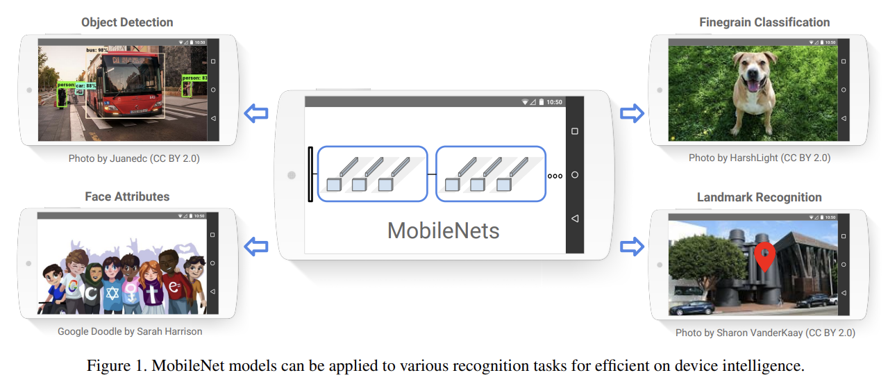
오늘 리뷰할 논문은 MobileNet이다. 가볍고 빨라서 모바일에서 자주 사용하는 모델이라고 들었다.

아래 포스트를 먼저 보면 도움이 될 것이다.

• MobileNet
• MobileNetV1 논문 설명(MobileNets - Efficient Convolutional Neural Networks for Mobile Vision Applications 리뷰)

---

논문은 mobile, embedded vision applications을 위해 효율적인 small, low latency network architecutre을 소개한다. 그리고 application의 resource restrictions (latency, size)를 만족하는 크기의 모델을 선택해 만들고자 set of two hyper-parameters를 사용한다.

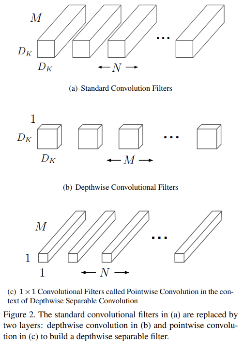
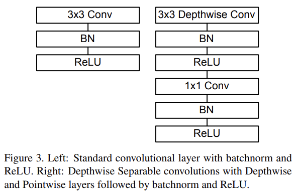
light weight를 위해 MobileNet은 기본적으로 depthwise separable convolutions를 사용하는 streamlined architecture에 기반한다. depthwise separable convolution이란 standard convolution를 depthwise convolution과 (pointwise convolution이라고 불리는) 1×1 convolution으로 factorize하는 일종의 factorized convolution이다. MobileNet의 depthwise convolution은 각 input channel에 filter를 하나씩 적용한다. 그 후 depthwise convolution의 outputs를 결합하기 위해 pointwise convolution이 1×1 convolution을 적용한다. standard convolution은 inputs을 new set of outputs로 one step에 동시에 filter하고 combine한다. 반면 depthwise separable convolution은 이를 두 layers로, filtering을 위한 layer와 combining을 위한 layer로 쪼갠다. 이 factorization은 연산량을 줄이고 모델 크기를 축소시키는 효과가 있다.

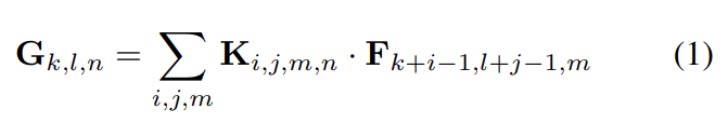
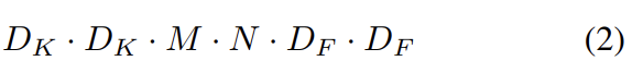
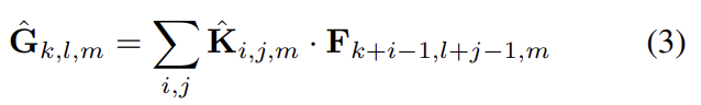
standard convolutional layer은 $D_F × D_F × M$ feature map F를 input으로 받아 $D_K × D_K × M × N$ 크기의 커널 K를 적용해 $D_F × D_F × N$ feature map G를 얻는다. convolution 연산은 식 (1)과 같이 되고 연산량은 식 (2)가 된다.

MobileNet은 우선 depthwise separable convolution을 사용해 output channels의 개수와 kernel size의 interaction을 부순다. depthwise convolution에서 input channel(=input depth)마다 single filter을 적용하고 pointwise convolution에서 simple 1×1 convolution을 사용해서 depthwise layer output의 linear combination을 생성한다. 두 layer 모두 batchnorm과 ReLU nonlinearities를 사용한다.

$D_K × D_K × M$ 크기의 m번째 커널 $\hat K$를 F의 m번째 channel에 적용해서 filtered output feature map $\hat G$의 m번째 channel을 만든다. Depthwise convolution의 연산과 연산량은 다음과 같다.

Depthwise convolution는 standard convolution에 비해 매우 효율적이다. 그러나 input channel을 filter할 뿐, 새로운 features를 조합한 것은 아니다. 그래서 pointwise convolution으로 linear combination를 계산해준다. 결과적으로 depthwise convolution(식 (2)에서 N=1)과 pointwise convolution(식 (2)에서 $D_K=1$)의 연산량을 합쳐 Depthwise separable convolution의 연산량은 아래와 같다.

MobileNet은 full convolution인 첫번째 layer을 제외하면 전부 depthwise separable convolution이다. nonlinearity가 없고 classification을 위한 softmax layer로 이어지는 final fully connected layer만 제외하면 모든 layer은 batchnorm과 ReLU nonlinearity가 뒤따른다.

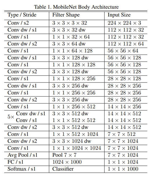
downsampling은 첫번째 layer와 depthwise convolutions에서의 strided convolution으로 이루어진다. final average pooling은 fully connected layer 직전에 spatial resolution을 1로 축소시킨다. depthwise, pointwise convolutions을 따로 세서 MobileNet은 28 layers로 이루어진다.

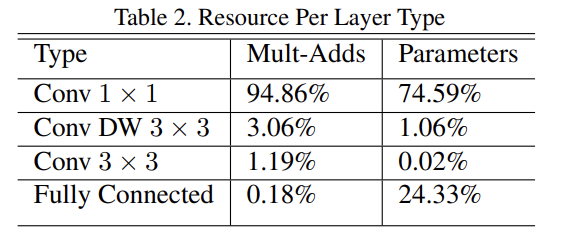
network 효율을 단순히 Mult-Adds 연산의 횟수로 정의하는 건 불충분하다. operations이 효율적으로 implementable한지도 중요하기 때문이다. 예컨대 unstructured sparse matrix operations은 sparsity가 아주 높지 않을 때까지 일반적으로 dense matrix operations보다 빠르지 않다. Table 2에서 볼 수 있듯 MobileNet은 거의 모든 연산을 dense 1 × 1 convolutions에 할당한다. 이는 highly optimized general matrix multiply (GEMM) functions로 구현될 수 있다.

MobileNet은 Inception V3와 비슷한 asynchronous gradient descen를 가진 RMSProp을 사용해서 TensorFlow로 학습됐다. 그러나 regularization와 data augmentation techniques를 적게 사용했는데 작은 모델은 overfitting 문제를 덜 겪기 때문이다. 학습시킬때 side heads나 label smoothing를 사용하지 않았고 large Inception training처럼 small crops의 크기를 제한하는 것으로 amount image of distortions를 감소시켰다. 추가로 depthwise filter에 (parameter가 너무 적기 때문에) weight decay (l2 regularization)를 아주 적거나 안 적용하는 것이 중요하다는 것을 발견했다.

이제 두 model shrinking hyperparameters인 width multiplier와 resolution multiplier에 대해 알아보자. Width Multiplier는 Thinner Model을 위해, Resolution Multiplier는 Reduced Representation을 위해 사용한다.

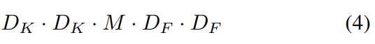
MobileNet의 architecture가 이미 samll하고 low latency이기는 한데 종종 특정 application에 사용하기 위해 크기가 더 작거나 더 빨라야할 수도 있다. 이를 위해 width multiplier이라고 이름붙인 parameter α를 도입한다. 이 파라미터의 역할은 network의 각 layer을 uniformly하게 thin하는 것이다. input channels M의 개수는 αM이 되고 output channels N의 개수는 αN가 되어 아래와 같이 depthwise separable convolution의 연산량이 변한다.

α ∈ (0, 1]이며 1, 0.75, 0.5, 0.25를 일반적으로 사용한다. α = 1를 baseline MobileNet, α < 1인 경우를 reduced MobileNets라고 부른다. width multiplier은 대략적으로 $α^2$로 quadratically하게 computational cost와 parameters 개수를 줄이는 효과가 있다. width multiplier은 어떤 model structure에도 적용될 수 있으며 합리적인 accuracy, latency, size tradeoff의 smaller model을 정의할 수 있다.

연산량 감소를 위해 두 번째로 소개할 hyperparameter은 resolution multiplier ρ이다. 이를 input image에 적용해서 결과적으로 모든 layer의 internal representation에 같은 multiplier에 의해 축소된다. 실제로는 input resolution을 setting하는 것으로 ρ를 implicit하게 설정한다. width multiplier와 resolution multiplier을 모두 적용한 연산량은 식 (7)과 같다.

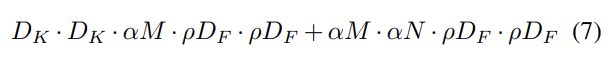
ρ ∈ (0, 1]이며 일반적으로 input resolution이 224, 192, 160, 128이도록 implicit하게 설정했다. 마찬가지로 ρ = 1이 baseline MobileNet이고 ρ < 1인 경우가 reduced computation MobileNets이다. resolution multiplier도 연산량을 $ρ^2$로 줄이는 효과가 있다.

실험은 우선 depthwise convolutions의 효과를 확인하고 다음으로 두 hyperparameter을 조절하며 tradeoff를 확인한다. 그리고 MobileNet을 여러 application에 적용해본다.

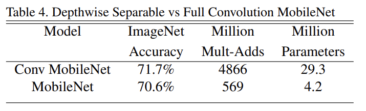
Table 4는 full convolution을 사용했을 때보다 depthwise separable convolution을 사용하는 게 정확도를 단 1%밖에 떨어뜨리지 않으면서 multi-adds 연산과 parameter은 극적으로 줄여줌을 보여준다.

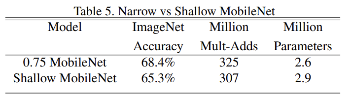
Table 5는 width multiplier을 사용한 thinner model과 (Table 1에서 feature size 14 × 14 × 512를 가진 5 layers of separable filters를 제거한) shallower model을 비교했다. 연산량과 parameter 수는 비슷한데 thinner한 것이 shallower한 것보다 정확도가 3% 좋음을 알 수 있다.

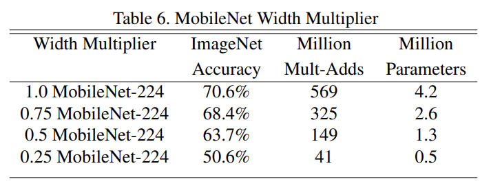
Table 6는 width multiplier로 network를 축소했을 때 accuracy, computation, size tradeoffs를 확인한 것이다. architecture가 0.25로 너무 작아지지 않는 이상 정확도가 smooth하게 떨어진다.

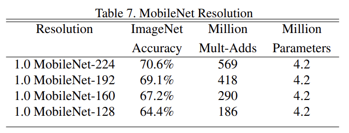
Table 7은 resolution multiplier에 따른 accuracy, computation, size tradeoffs 결과다. resolution 축소에 따라 정확도가 smooth하게 떨어진다.

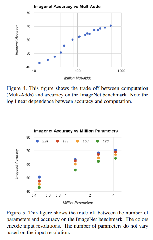
Fig 4, 5는 width multiplier α ∈ {1, 0.75, 0.5, 0.25}와 resolutions {224, 192, 160, 128}을 cross product한 16 model에서 ImageNet Accuracy와 computation, parameters 수 tradeoff를 확인한 것이다.

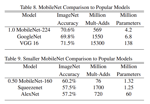
Table 8, 9는 여러 유명한 모델들과 MobileNet을 비교한 것이다.

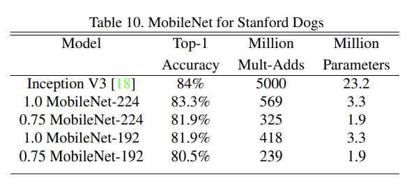
MobileNet을 Stanford Dogs 데이터셋에 학습시켜 fine grained recognition 능력을 확인했다. 크게 감소한 computation과 size로 SOTA 결과를 얻을 수 있었다.

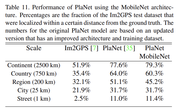
PlaNet은 사진이 지구 상 어느 위치에서 찍혔는지 결정하는 classification 과제를 다룬다. 논문은 PlaNet을 MobileNet으로 재학습시켜 훨씬 크기가 작으면서 성능은 조금만 떨어지는 결과를 얻었다.

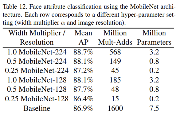
MobileNet의 또 다른 용법은 unknown/esoteric training procedures를 지닌 large systems을 압축하는 것이다. face attribute classification task에서 MobileNet과 deep network의 knowledge transfer technique인 distillation의 관계를 입증한다. Distillation은 classifier가 ground-truth label을 학습하는 대신 larger model의 output을 emulate하도록 학습시킨다. Table 12에서 MobileNet-based classifier는 aggressive model shrinking에 resilient한 모습을 보인다.

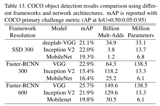
MobileNet은 object detection systems의 base network로도 효과적이다. Table 13은 Faster R-CNN과 SSD framework 하에서 MobileNet, VGG, Inception V2를 비교한 결과다. 두 framework 모두에서 MobileNet이 적은 연산량과 크기만으로도 경쟁력있는 성능을 보였다.

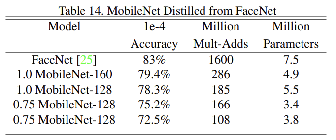
FaceNet은 triplet loss에 기반해 face embeddings을 만드는 SOTA face recognition model이다. mobile FaceNet model을 만들기 위해 distillation을 사용해서 training data에 대한 FaceNet과 MobileNet의 output 사이 squared differences을 최소화하도록 학습했다. 결과는 Table 14와 같다.

Strengths

1. width mutliplier와 resolution multiplier을 통해 모델의 연산량 및 크기 변화에 유연성을 줬다. layer 수를 줄이는 것보다 width를 줄이는 게 더 효율적임을 보인 것도 좋았다. (그런데 사실 이론적으로 그렇게 의미있는 하이퍼파라미터는 아닌 것 같고 그냥 네트워크의 width와 resolution 설정을 기호로 명시화?한 것 뿐인 듯하다)
2. depthwise separable convolution의 아이디어가 단순하면서도 강력했다. VGGNet에서 큰 필터 대신 3x3 필터 여러 개를 겹쳐 더 적은 파라미터로 좋은 성능을 낸 것과 같은 맥락인 것 같다. 모델 연산량/크기의 극적인 감소에 비해 성능 하락은 거의 없어서 결과가 몹시 인상적이었다.
3. MobileNet이 distillation에 효과가 좋은 점이 유용하게 느껴졌다.