• Pandas was originally developed in the context of financial modeling, so it contains an extensive set of tools for working dates, times, and time-indexed data.
• Timestamps : Particular moments in time
• Time interval and periods : A length of time between a particular beginning and end point
• Time deltas or durations : An exact length of time

Dates and Times in Python

Native Python Dates and Times: datetime and dateutil

# In[1]
from datetime import datetime
datetime(year=2023,month=7,day=28)

# Out[1]
datetime.datetime(2023, 7, 28, 0, 0)

• Or, using the dateutil module, you can parse dates from a variety of string formats.

# In[2]
from dateutil import parser
date=parser.parse("28th of July, 2023")
date

# Out[2]
datetime.datetime(2023, 7, 28, 0, 0)

• Using datetime object, you can do things like printing the day of the week.

# In[3]
date.strftime('%A')

# Out[3]
'Friday'

Typed Arrays of Times: Numpy's datetime64

• Numpy's datetime64 dtype encodes dates as 64-bit integers, and thus allows arrays of dates to be represented compactly and operated on in an efficient manner.
• It requires a specific input format

# In[4]
date=np.array('2023-07-28',dtype=np.datetime64)
date

# Out[4]
array('2023-07-28', dtype='datetime64[D]')

• We can quickly do vectorized operations on it.

# In[5]
date+np.arange(12)

# Out[5]
array(['2023-07-28', '2023-07-29', '2023-07-30', '2023-07-31',
       '2023-08-01', '2023-08-02', '2023-08-03', '2023-08-04',
       '2023-08-05', '2023-08-06', '2023-08-07', '2023-08-08'],
      dtype='datetime64[D]')

• This kind of operation can be accomplished much more quickly than if we were working directly with Python's datetime objects, especially as arrays get large.

---

• One detail of the datetime64 and related timedelta64 objects is that they are built on a fundamental time unit.
• The datetime64 object is limited to 64-bit precision, the range of encodable times is $2^{64}$ times this fundamental unit.
• datetime64 imposes a trade-off between time resolution and maximum time span.

# In[6]
print(np.datetime64('2023-07-28')) # day based
print(np.datetime64('2023-07-28 12:00')) # minute based
print(np.datetime64('2023-07-28 12:59:59.50','ns')) # nanosecond based

# Out[6]
2023-07-28
2023-07-28T12:00
2023-07-28T12:59:59.500000000

• More informations about datetime64 can be found in Numpy's datatime64 documentation

Dates and Times in Pandas: The Best of Both Worlds

• Pandas builds upon all the tools just discussed to provide a Timestamp object, which combines the ease of use of datetime and dateutil with the efficient storage and vectorized interface of numpy.datetime64
• From a group of these Timestamp objects, Pandas can construct a DatetimeIndex that can be used to index data in a Series or DataFrame.

# In[7]
date=pd.to_datetime("28th of July, 2023")
date

# Out[7]
Timestamp('2023-07-28 00:00:00')

---

# In[8]
date.strftime('%A')

# Out[8]
'Friday'

• We can do Numpy-style vectorized operations directly on this same object.

# In[9]
date+pd.to_timedelta(np.arange(12),'D')

# Out[9]
DatetimeIndex(['2023-07-28', '2023-07-29', '2023-07-30', '2023-07-31',
               '2023-08-01', '2023-08-02', '2023-08-03', '2023-08-04',
               '2023-08-05', '2023-08-06', '2023-08-07', '2023-08-08'],
              dtype='datetime64[ns]', freq=None)

Pandas Time Series: Indexing by Time

• The Pandas time series tools really become useful when you begin to index date by timestamps.

# In[10]
index=pd.DatetimeIndex(['2023-07-28','2023-08-28',
'2024-07-28','2024-08-28'])
data=pd.Series([0,1,2,3],index=index)
data

# Out[10]
2023-07-28    0
2023-08-28    1
2024-07-28    2
2024-08-28    3
dtype: int64

• We can make use of any of the Series indexing patterns, passing values that can be coerced(=force) into dates.

# In[11]
data['2023-07-28':'2024-07-28']

# Out[11]
2023-07-28    0
2023-08-28    1
2024-07-28    2
dtype: int64

• There are additional special date-only indexing operations, such as passing a year to obtain a slice of all data from that year.

# In[12]
data['2023']

# Out[12]
2023-07-28    0
2023-08-28    1
dtype: int64

Pandas Time Series: Data Structure

• For timestamps, Pandas provides the Timestamp type.

  • This is essentially a replacement for Python's native datetime, but it's based on the more effcient np.datetime64 data type.
  • Associated Index structure is DatetimeIndex

• For time periods, Pandas provides the Period type.

  • This encodes a fixed-frequency interval based on np.datetime64
  • Associated index structure is PeriodIndex

• For time deltas or durations, Pandas provides the Timedelta type.

  • It is a more efficient replacement for Python's native datetime.timedelta type, and is based on np.timedelta64
  • Associated index structure is TimedeltaIndex

• Commonly, we use the pd.to_datetime function, which can parse(=analyze) a wide variety of formats.

• Passing a single date to pd.to_datetime yields a Timestamp.

# In[13]
dates=pd.to_datetime([datetime(2023,7,28),'28th of July, 2023',
'2023-07-30','31-07-2023','20230801'])
dates

# Out[13]
DatetimeIndex(['2023-07-28', '2023-07-28', '2023-07-30', '2023-07-31',
               '2023-08-01'],
              dtype='datetime64[ns]', freq=None)

• Any DatetimeIndex can be converted to a PeriodIndex with the to_period function, with the addition of a frequency code.

# In[14]
dates.to_period('D')

# Out[14]
PeriodIndex(['2023-07-28', '2023-07-28', '2023-07-30', '2023-07-31',
             '2023-08-01'],
            dtype='period[D]')

• A TimedeltaIndex is created when a date is subtracted from another.

# In[15]
dates-dates[0]

# Out[15]
TimedeltaIndex(['0 days', '0 days', '2 days', '3 days', '4 days'], dtype='timedelta64[ns]', freq=None)

Regular Sequences: pd.date_range

• To make creation of regular date sequences more convenient, Pandas offers a few functions for this purpose
• pd.date_range for timestamps
• pd.period_range for periods
• pd.timedelta_range for time deltas.

# In[16]
pd.date_range('2023-07-28','2023-08-14')

# Out[16]
DatetimeIndex(['2023-07-28', '2023-07-29', '2023-07-30', '2023-07-31',
               '2023-08-01', '2023-08-02', '2023-08-03', '2023-08-04',
               '2023-08-05', '2023-08-06', '2023-08-07', '2023-08-08',
               '2023-08-09', '2023-08-10', '2023-08-11', '2023-08-12',
               '2023-08-13', '2023-08-14'],
              dtype='datetime64[ns]', freq='D')

• The date range can be specified not with a start and end point, but with a start point and a number of periods.

# In[17]
pd.date_range('2023-07-28',periods=8)

# Out[17]
DatetimeIndex(['2023-07-28', '2023-07-29', '2023-07-30', '2023-07-31',
               '2023-08-01', '2023-08-02', '2023-08-03', '2023-08-04'],
              dtype='datetime64[ns]', freq='D')

• The spacing can be modified by altering the freq argument, which defaults to D.

# In[18]
pd.date_range('2023-07-28',periods=8,freq='H')

# Out[18]
DatetimeIndex(['2023-07-28 00:00:00', '2023-07-28 01:00:00',
               '2023-07-28 02:00:00', '2023-07-28 03:00:00',
               '2023-07-28 04:00:00', '2023-07-28 05:00:00',
               '2023-07-28 06:00:00', '2023-07-28 07:00:00'],
              dtype='datetime64[ns]', freq='H')

• To create regular sequence of Period or Timedelta values, the similar pd.period_range and pd.timedelta_range functions are useful.

# In[19]
pd.period_range('2023-07',periods=8,freq='M')

# Out[19]
PeriodIndex(['2023-07', '2023-08', '2023-09', '2023-10', '2023-11', '2023-12',
             '2024-01', '2024-02'],
            dtype='period[M]')

---

# In[20]
pd.timedelta_range(0,periods=6,freq='H')

# Out[20]
TimedeltaIndex(['0 days 00:00:00', '0 days 01:00:00', '0 days 02:00:00',
                '0 days 03:00:00', '0 days 04:00:00', '0 days 05:00:00'],
               dtype='timedelta64[ns]', freq='H')

Frequencies and Offsets

• Fundamental to these Pandas time series tools is the concept of a frequency or date offset.

Listing of Pandas frequency codes

Code	Description	Codes	Description
D	Calendar day	B	Business day
W	Weekly
M	Month end	BM	Business month end
Q	Quarter end	BQ	Business quarter end
A	Year end	BA	Business year end
H	Hours	BH	Business hours
T	Minutes
S	Seconds
L	Milliseconds
U	Microseconds
N	Nanoseconds

• The monthly, quarterly, and annual frequencies are all marked at the end of the specified period.

Listing of start-indexed frequency codes

Code	Description
MS	Month start
QS	Quarter start
AS	Year start
BS	Business month start
BQS	Business quarter start
BAS	Business year start

• Additionally, you can change the month used to mark any quarterly or annual code by adding a three-letter month code as a suffix.

  • Q-JAN, BQ-FEB, QS-MAR, BQS-APR etc.

• In the same way, the split point of the weekly frequency can be modified by adding a three-letter weekday code.

  • W-SUN, W-MON, W-TUE, W-WED etc.

• Codes can be combined with numbers to specify otehr frequencies.

# In[21]
pd.timedelta_range(0,periods=6,freq='2H30T')

# Out[21]
TimedeltaIndex(['0 days 00:00:00', '0 days 02:30:00', '0 days 05:00:00',
                '0 days 07:30:00', '0 days 10:00:00', '0 days 12:30:00'],
               dtype='timedelta64[ns]', freq='150T')

• All of these short codes refer to specific instances of Pandas time series offsets, which can be found in the pd.tseries.offsets module.

# In[22]
from pandas.tseries.offsets import BDay
pd.date_range('2023-07-28',periods=6,freq=BDay())

# Out[22]
DatetimeIndex(['2023-07-28', '2023-07-31', '2023-08-01', '2023-08-02',
               '2023-08-03', '2023-08-04'],
              dtype='datetime64[ns]', freq='B')

• For more information about the use of frequencies and offsets, see the DateOffset section of the Pandas documentation

Resampling, Shifting, and Windowing

• The ability to use dates and times as indices to intuitively organize and access data is an important aspect of the Pandas time series tools.
• The benefits of indexed data in general still apply, and Pandas provides several additional time series-specific operations.

# In[23]
import pandas_datareader.data as web
start_date = datetime(2006, 1, 1)
end_date = datetime(2016, 1, 1)
#Bank of America
bac = data.DataReader('BAC', 'stooq', start_date, end_date)
bac.head()

# Out[23]
               Open	   High	    Low	  Close	      Volume
Date					
2015-12-31	14.7814	14.8325	14.6233	14.6233	5.417059e+07
2015-12-30	14.9473	14.9807	14.8070	14.8168	4.030734e+07
2015-12-29	14.9897	15.0780	14.9130	15.0131	5.251059e+07
2015-12-28	14.9630	14.9720	14.7539	14.8846	4.803435e+07
2015-12-24	15.0495	15.1035	14.9630	15.0063	3.380344e+07

---

# In[24]
bac=bac['Close']

• We can visualize this using the plot method.

# In[25]
%matplotlib inline
import matplotlib.pyplot as plt
plt.style.use('seaborn-whitegrid')
bac.plot();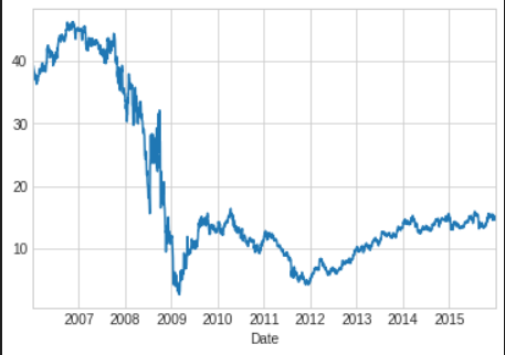

Resampling and Converting Frequencies

• One common need when dealing with time series data is resampling at a higher or lower frequency.
• This can be done using the resample method, or the much simpler asfreq method.
• The primary difference between the two is that resample is fundamentally a data aggregation, while asfreq is fundamentally a data selection.

# In[26]
bac.plot(alpha=0.5,style='-')
bac.resample('BA').mean().plot(style=':')
bac.asfreq('BA').plot(style='--')
plt.legend(['input','resample','asfreq'],loc='upper left');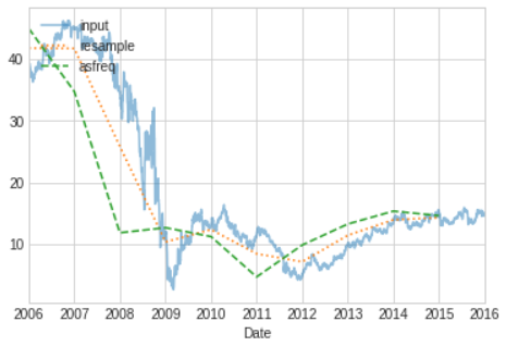

• resample reports the average of the previous year, while asfreq reports the value at the end of the year.
  
  
• For upsampling, resample and asfreq are largely equivalent, though resample has many more options available.
• Like the pd.fillna function, asfreq accepts a method argument to specify how values are imputed.

# In[27]
fig, ax=plt.subplots(2,sharex=True)
data=bac.iloc[:20]

data.asfreq('D').plot(ax=ax[0],marker='o')

data.asfreq('D',method='bfill').plot(ax=ax[1],style='-o')
data.asfreq('D',method='ffill').plot(ax=ax[1],style='--o')
ax[1].legend(["back-fill","forward-fill"]);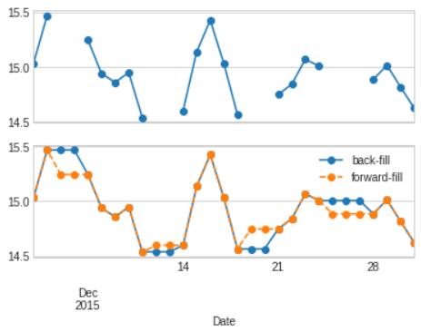

• The bottom panel shows the differences between two strategies for filling the gaps: forward filling and backward filling

Time Shifts

• Another common tine series-specific operation is shifting of data in time.
• For this, Pandas provides the shift method, which can be used to shift data by a given number of entries.

# In[28]
bac=bac.asfreq('D',method='pad')
ROI=100*(bac.shift(-365)-bac)/bac
ROI.plot()
plt.ylabel('%  Return on Investment after 1 year');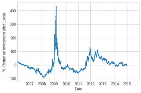

Rolling Windows

• Calculating rolling statistics is a third type of time series-specific operation implemented by Pandas.
• This can be accomplished via the rolling attribute of Series and DataFrame object, which returns a view similar to what we saw with the groupby operation.
• This rolling view makes available a number of aggregation operations by default.

# In[29]
rolling=bac.rolling(365,center=True)
data=pd.DataFrame({'input':bac,'one-year rolling_mean':rolling.mean(),
'one-year rolling_median':rolling.median()})
ax=data.plot(style=['-','--',':'])
ax.lines[0].set_alpha(0.3)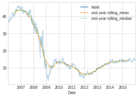

• As with groupby operations, the aggregate and apply methods can be used for custom rolling computations.
  
  
• For a more complete discussion, you can refer to the
  Time Series/Date Functionality section of the Pandas online documentation