# In[1]
class display(object):
    """Display HTML representation of multiple objects"""
    template="""<div style="float: left; padding: 10px;">
    <p style='font-family:"Courier New", Courier, monospace'>{0}{1}
    """
    def __init__(self,*args):
        self.args=args
    
    def _repr_html_(self):
        return '\n'.join(self.template.format(a,eval(a)._repr_html_()) 
                         for a in self.args)
    
    def __repr__(self):
        return '\n\n'.join(a+'\n'+repr(eval(a))
                         for a in self.args)

Planets Data

• We will use Planets dataset, available via the Seaborn package.
• Planets Dataset gives information on planets that astronomers have discovered around other stars.

# In[2]
import seaborn as sns
planets=sns.load_dataset('planets')
planets.shape

# Out[2]
(1035, 6)

---

# In[3]
planets.head()

# Out[3]
             method	number	orbital_period	 mass	distance	year
0	Radial Velocity	     1	      269.300	 7.10	   77.40	2006
1	Radial Velocity	     1	      874.774	 2.21	   56.95	2008
2	Radial Velocity	     1	      763.000	 2.60	   19.84	2011
3	Radial Velocity	     1	      326.030	19.40	  110.62	2007
4	Radial Velocity	     1	      516.220	10.50	  119.47	2009

Simple Aggregation in Pandas

• As with a one-dimensional Numpy array, for a Pandas Series the aggregates return a single value.

# In[4]
rng=np.random.RandomState(42)
ser=pd.Series(rng.rand(5))
ser

# Out[4]
0    0.374540
1    0.950714
2    0.731994
3    0.598658
4    0.156019
dtype: float64

---

# In[5]
ser.sum()

# Out[5]
2.811925491708157

---

# In[6]
ser.mean()

# Out[6]
0.5623850983416314

• For a DataFrame, by default the aggregates return results within each column.

# In[7]
df=pd.DataFrame({'A':rng.rand(5),'B':rng.rand(5)})
df

# Out[7]
           A	       B
0	0.155995	0.020584
1	0.058084	0.969910
2	0.866176	0.832443
3	0.601115	0.212339
4	0.708073	0.181825

---

# In[8]
df.mean()

# Out[8]
A    0.477888
B    0.443420
dtype: float64

---

# In[9]
df.mean(axis=1)

# Out[9]
0    0.088290
1    0.513997
2    0.849309
3    0.406727
4    0.444949
dtype: float64

• Pandas Series and DataFrame objects include all of the common aggregates.
• There is a convenience method, describe, that computes several common aggregates for each column and returns the result.

# In[10]
planets.dropna().describe()

# Out[10]
           number	orbital_period	      mass	  distance	       year
count	498.00000	    498.000000	498.000000	498.000000	 498.000000
mean	  1.73494	    835.778671	  2.509320	 52.068213	2007.377510
std	      1.17572	   1469.128259	  3.636274	 46.596041	   4.167284
min	      1.00000	      1.328300	  0.003600	  1.350000	1989.000000
25%	      1.00000	     38.272250	  0.212500	 24.497500	2005.000000
50%	      1.00000	    357.000000	  1.245000	 39.940000	2009.000000
75%	      2.00000	    999.600000	  2.867500	 59.332500	2011.000000
max	      6.00000	  17337.500000	 25.000000	354.000000	2014.000000

• This method helps us understand the overall properties of a dataset.

Listing of Pandas aggregation methods

Aggregation	Returns
count	Total number of items
first, last	First and last item
mean, median	Mean and median
min, max	Minimum and maximum
std, var	Standard deviation and variance
mad	Mean absolute deviation
prod	Product of all items
sum	Sum of all items

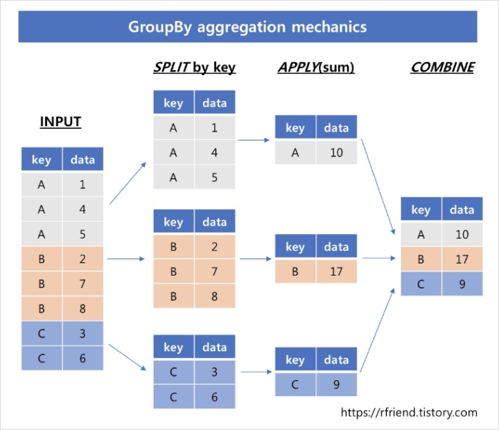
groupby: Split, Apply, Combine

Split, Apply, Combine

• The split step involves breaking up and grouping a DataFrame depending on the value of the specified key.
• The apply step involves computing some function, usually an aggregate, tranformation, or filtering, within the individual groups.
• The combine step merges the results of these operations into an output array.

• While this could certainly be done manually using some combination of the masking, aggregation, and merging commands covered earlier, an important realization is that the intermediate splits do not need to be explicitly instantiated.
• Rather, the groupby can do this in a single pass over the data, updating sum, mean, count, min, or other aggregate for each group along the way.
• The user need not think about how the computation is done under the hood, but rather can think about the operation as a whole.

# In[11]
df=pd.DataFrame({'key':['A','B','C','A','B','C'],
'data':range(6)},columns=['key','data'])
df

# Out[11]
  key	data
0	A	   0
1	B	   1
2	C	   2
3	A	   3
4	B	   4
5	C	   5

• The most basic split-apply-combine operation can be computed with the groupby method of DataFrame, passing the name of the desired key column.

# In[12]
df.groupby('key')

# Out[12]
<pandas.core.groupby.generic.DataFrameGroupBy object at 0x7fb7844dd240>

• To produce a result, we can apply an aggregate to this DataFrameGroupBy object, which will perform the appropriate apply/combine step to produce the desired result.

# In[13]
df.groupby('key').sum()

# Out[13]
    data
key	
A	   3
B	   5
C	   7

The GroupBy Object

• The GroupBy object is a flexible abstraction: in many ways, it can be treated as simply a collection of DataFrames, though it is doing more sophisticated things under the hood.

Column indexing

• The GroupBy object supports column indexing in the same way as the DataFrame, and returns a modified GroupBy object.

# In[14]
planets.groupby('method')

# Out[14]
<pandas.core.groupby.generic.DataFrameGroupBy object at 0x7fb7844dd2a0>

---

# In[15]
planets.groupby('method')['orbital_period']

# Out[15]
<pandas.core.groupby.generic.SeriesGroupBy object at 0x7fb7844dcd60>

• We've selected a particular Series group from the original DataFrame group by reference to its column name.
• As with the GroupBy object, no computation is done until we call some aggregate on the object.

# In[16]
planets.groupby('method')['orbital_period'].median()

# Out[16]
method
Astrometry                         631.180000
Eclipse Timing Variations         4343.500000
Imaging                          27500.000000
Microlensing                      3300.000000
Orbital Brightness Modulation        0.342887
Pulsar Timing                       66.541900
Pulsation Timing Variations       1170.000000
Radial Velocity                    360.200000
Transit                              5.714932
Transit Timing Variations           57.011000
Name: orbital_period, dtype: float64

Iteration over groups

• The GroupBy object supports direct iteration(반복) over the groups, returning each group as a Series or DataFrame.

# In[17]
for (method,group) in planets.groupby('method'):
    print("{0:30s} shape={1}".format(method,group.shape))

# Out[17]
Astrometry                     shape=(2, 6)
Eclipse Timing Variations      shape=(9, 6)
Imaging                        shape=(38, 6)
Microlensing                   shape=(23, 6)
Orbital Brightness Modulation  shape=(3, 6)
Pulsar Timing                  shape=(5, 6)
Pulsation Timing Variations    shape=(1, 6)
Radial Velocity                shape=(553, 6)
Transit                        shape=(397, 6)
Transit Timing Variations      shape=(4, 6)

• It is often much faster to use the built-in apply functionality.

Dispatch methods

• Though some Python class magic, any method not explicitly implemented by the GroupBy object will be passed through and called on the groups, whether they are DataFrame or Series objects.

# In[18]
planets.groupby('method')['year'].describe().unstack()

# Out[18]
       method                       
count  Astrometry                          2.0
       Eclipse Timing Variations           9.0
       Imaging                            38.0
       Microlensing                       23.0
       Orbital Brightness Modulation       3.0
                                         ...  
max    Pulsar Timing                    2011.0
       Pulsation Timing Variations      2007.0
       Radial Velocity                  2014.0
       Transit                          2014.0
       Transit Timing Variations        2014.0
Length: 80, dtype: float64

• dispatch methods are applied to each individual group, and the results are then combined within GroupBy and returned.
• Any valid DataFrame/Series method can be called in a similar manner on the corresponding GroupBy object.

Aggregate, Filter, Transform, Apply

• The preceding discussion focused on aggregation for the combine operation, but there are more options available.
• In particular, GroupBy objects have aggregate, filter, transform, and apply methods that efficiently implement a variety of useful operations before combining the grouped data.

# In[19]
rng=np.random.RandomState(0)
df=pd.DataFrame({'key':['A','B','C','A','B','C'],
'data1':range(6), 'data2':rng.randint(0,10,6)},columns=['key','data1','data2'])
df

# Out[19]
  key data1	data2
0	A	  0	    5
1	B	  1	    0
2	C	  2	    3
3	A	  3	    3
4	B	  4	    7
5	C	  5	    9

Aggregation

• You're now familiar with GroupBy aggregations with sum, median, and the like, but the aggregate method allows for even more flexibility.
• It can be a string, a function, or a list thereof, and compute all the aggregates at once.

# In[20]
df.groupby('key').aggregate(['min',np.median,max])

# Out[20]
   data1	        data2
   min	median	max	min	median	max
key						
A	 0	   1.5	  3	  3	  4.0	  5
B	 1	   2.5	  4	  0	  3.5	  7
C	 2	   3.5	  5	  3	  6.0	  9

• Another common pattern is to pass a dictionary mapping column names to operations to be applied on that column.

# In[21]
df.groupby('key').aggregate({'data1':'min','data2':'max'})

# Out[21]
    data1	data2
key		
A	    0	    5
B	    1	    7
C	    2	    9

Filtering

• A filtering operation allows you to drop data based on the group properties.

# In[22]
def filter_func(x):
    return x['data2'].std()>4
display('df',"df.groupby('key').std()","df.groupby('key').filter(filter_func)")

# Out[22]
df

  key	data1	data2
0	A	    0	    5
1	B	    1	    0
2	C	    2	    3
3	A	    3	    3
4	B	    4	    7
5	C	    5	    9

df.groupby('key').std()

    data1	data2
key		
A	2.12132	1.414214
B	2.12132	4.949747
C	2.12132	4.242641

df.groupby('key').filter(filter_func)

  key	data1	data2
1	B	    1	    0
2	C	    2	    3
4	B	    4	    7
5	C	    5	    9

• The filter function should return a Boolean value specifying whether the group passes the filtering.

Transformation

• While aggregation must return a reduced version of data, transformation can return some transformed version of the full data to recombine.
• For such a transformation, the output is the same shape as the input.

# In[23]
def center(x):
    return x-x.mean()
df.groupby('key').transform(center)

# Out[23]
   data1	data2
0	-1.5	  1.0
1	-1.5	 -3.5
2	-1.5	 -3.0
3	 1.5	 -1.0
4	 1.5	  3.5
5	 1.5	  3.0

The apply method

• Lets you apply an arbitrary function to the group results.
• The function should take DataFrame and returns either a Pandas object or a scalar.

# In[24]
def norm_by_data2(x):
	# x is a DataFrame of group values 
    x['data1']/=x['data2'].sum()
    return x
df.groupby('key').apply(norm_by_data2)

# Out[24]
  key	   data1	data2
0	A	0.000000	    5
1	B	0.142857	    0
2	C	0.166667	    3
3	A	0.375000	    3
4	B	0.571429	    7
5	C	0.416667	    9

• apply within a GroupBy is flexible; the only criterion is that the function takes a DataFrame and returns a Pandas object or scalar.

Specifying the Split Key

A list, array, series, or index providing the grouping keys

• The key can be any series or list with a length matching that of the DataFrame.

# In[25]
L=[0,1,0,1,2,0]
df.groupby(L).sum()

# Out[25]
  data1	data2
0	  7	   17
1	  4 	3
2	  4	    7

---

# In[26]
df.groupby(df['key']).sum()

# Out[26]
    data1	data2
key		
A	    3	    8
B	    5	    7
C	    7	   12

A dictionary or series mapping index to group

• Provide a dictionary that maps index values to the group keys.

# In[27]
df2=df.set_index('key')
mapping={'A':'vowel','B':'consonant','C':'consonant'}
display('df2','df2.groupby(mapping).sum()')

# Out[27]
df2

    data1	data2
key		
A	    0	    5
B	    1	    0
C	    2	    3
A	    3	    3
B	    4	    7
C	    5	    9

df2.groupby(mapping).sum()

         data1	data2
key		
consonant	12	   19
vowel	     3	    8

Any Python function

• Similar to mapping, you can pass any Python function that will input the index value and output the group.

# In[28]
df2.groupby(str.lower).mean()

# Out[28]
    data1	data2
key		
a	  1.5	  4.0
b	  2.5	  3.5
c	  3.5	  6.0

A list of valid keys

• Any of the preceding key choices can be combined to group on a multi-index

# In[29]
df2.groupby([str.lower,mapping]).mean()

# Out[29]
              data1	data2
key	key		
a	    vowel	1.5	  4.0
b	consonant	2.5	  3.5
c	consonant	3.5	  6.0

Grouping Example

# In[30]
decade=10*(planets['year']//10)
decade=decade.astype(str)+'s'
decade.name='decade'
planets.groupby(['method',decade])['number'].sum().unstack().fillna(0)

# Out[30]
decade	                      1980s	1990s	2000s	2010s
method				
Astrometry	                    0.0	  0.0	  0.0	  2.0
Eclipse Timing Variations	    0.0	  0.0	  5.0	 10.0
Imaging	                        0.0	  0.0	 29.0	 21.0
Microlensing	                0.0	  0.0	 12.0	 15.0
Orbital Brightness Modulation	0.0	  0.0	  0.0	  5.0
Pulsar Timing	                0.0	  9.0	  1.0	  1.0
Pulsation Timing Variations	    0.0	  0.0	  1.0	  0.0
Radial Velocity	                1.0	 52.0	475.0	424.0
Transit	                        0.0	  0.0	 64.0	712.0
Transit Timing Variations	    0.0	  0.0	  0.0	  9.0