Formal Algorithms for Transformers 요약

주의 사항

• Transformer를 알고있다는 가정하에 글을 진행합니다.
• 이 글은 논문에 대한 요약글입니다.
• 논문 전체 내용 + Reference + Appendix를 함께 공부하시면 좋습니다.

Introduction

본 논문에서는 Transformers에 대한 complete, precise, and compact overview를 제공하는 것을 목적으로 Transformer components의 pseudocode를 소개하고 있습니다.

• what Transformers are (Section 6)
• how they are trained (Section 7)
• what they’re used for (Section 3)
• their key architureral components (Section 5)
• tokenization (Section 4)
• a preview of practical considerations (Section 8)
• the most preminent models

Encoder-only Transfomer, Decoder-only Transformer에 대한 algorithm과 함께 train, inference에 대한 algorithm도 같이 소개하고 있으니 함께 살펴보셔도 좋을 것 같습니다.

Notations

Notation

논문에서 쓰이는 notation에 대해 소개합니다. Appendix B에 Notation 목록이 포함되어있습니다.

• $[N] \coloneqq \{1,2,\dots, N-1, N\}$, $1\sim N$까지 정수를 포함한 집합
• $N_V$: vocabulary size
• $V \cong [N_V]$: vocabulary
• $V^* = \bigcup_{l=0}^{\infty}V^l$: vocabuary로 만들 수 있는 모든 sequence를 가지는 집합
• $l$: sequence length
  • $l_{max}$: maximum sequence length
• $x$: primary token sequence
  • $x_n \equiv x[1:l] \equiv x[1]x[2]\dots x[l] \in V^*$
  • $x[t]$: $x$의 $t$번째 token
  • Python과 달리 index의 시작이 1 입니다.
  • target이라는 표현을 사용하기도 하지만 여기서는 primary로 표기합니다.
• $z$: context token sequence, $x$에 대한 context sequence
  • $z_n \equiv z[1:l] \equiv z[1]z[2]\dots z[l] \in V^*$
  • $z[t]$: $z$의 $t$번째 token
  • Python과 달리 index의 시작이 1 입니다.
  • source라는 표현을 사용하기도 하지만 여기서는 context로 표기합니다.
• $M \in \R^{d \times d^\prime}$: matrix
  • $M[i,j]$ : entry $M_{ij}$
  • $M[i,:]$ : $M$의 $i$번째 row vector
  • $M[:,j]$ : $M$의 j번째 column vector
• $N_{data}$: data 갯수
• $n \in [N_{data}]$: n번째 data
  • $x_n$, $z_n$

Matrix Multiplication

• DL에서 많이 쓰이는 row vector $\times$ matrix 대신 수학에서 자주 쓰이는 matrix $\times$ column vector를 사용합니다.
  • 따라서 각각의 component에서 반환되는 vector는 모두 column vector로 표시됩니다.

Final Vocabulary and text representation

• Tokenization을 통해 만든 vocabulary에 3가지 special token을 추가하여 final vocabulary를 만듭니다.
• special token을 제외한 나머지 token들에 대해서 $\{1,2,\dots, N_V-3\}$의 unique index를 할당합니다.
• special token은 다음과 같습니다.
  • $\text{mask\_token} \coloneqq N_V-2$, masked language modelling에 쓰이는 token
  • $\text{bos\_token} \coloneqq N_V-1$, the beginning of sequence, sequence의 시작을 알리는 token
  • $\text{eos\_token} \coloneqq N_V$, the end of sequence, sequence의 마지막을 알리는 token

Algorithm 1: Token embedding

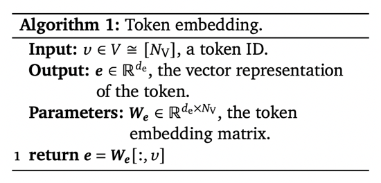
Input

• $v$: token ID

Output

• $e \in \R^{d_e}$: 입력으로 들어온 token ID에 대한 embedding vector 반환.

Parameters

• $W_e \in \R^{d_e\times N_V}$: embedding matrix
  • vocabulary에 존재하는 모든 token에 대해 embedding 값을 반환하기 위해서 column size가 $N_V$가 됩니다.

과정

• 1번: token ID $v$에 대한 vector representation을 반환합니다.

Algorithm 2: Positional embedding

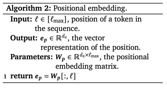
Attention is All You Need에서는 고정된 Positional Encoding 사용하지만 이 논문에서는 Postional Encoding 또한 학습 parameter로 설정하였습니다.

Input

• $l$: position in sequence

Output

• $e \in \R^{d_e}$: 입력으로 들어온 postion에 대한 embedding vector 반환.

Parameters

• $W_e \in \R^{d_e\times l_{max}}$: positional embedding matrix
  • data에 존재하는 모든 sequence에 대해 positional embedding 값을 반환하야하기 때문에 column size가 $l_{max}$가 됩니다.

과정

• 1번: position $l$에 대한 vector representation가 됩니다.

최종적으로 sequence $x$의 $t$번째 token에 대한 embedding vector는 다음과 같습니다.

• $e = W_e[:,x[t]] + W_p[:,t]$

Algorithm 3: Basic single-query attention

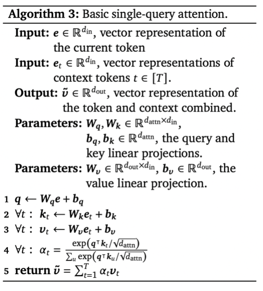
Attention is all You Need 논문에 소개된 single query attention 과정인 $A(q,K,V) = \sum\limits_i \frac{exp(q \cdot k_i)}{\sum_j exp(q \cdot k_j)} v_i$ 을 그대로 적용합니다.

Input

• $e\in\R^{d_{in}}$: 현재 token에 대한 vector representation
• context sequence에 존재하는 모든 token에 대한 vector representation
  • $e_t\in\R^{d_{in}}$: context sequence의 $t$번째 token에 대한 vector representation

Output

• 현재 token과 context 정보를 결합한 vector representation 반환
  • $\tilde{v} \in \R^{d_{out}}$
• 실제 Transformer에서는 attention 이후 residual connection을 하기 때문에 이 점에 유의해서 $d_{out}$과 $d_{in}$를 설정해주어야합니다.

Parameters

• $W_e \in \R^{d_{attn}\times d_{in}}$: query linear projection
  • $b_e \in \R^{d_{attn}}$: bias term
• $W_k \in \R^{d_{attn}\times d_{in}}$: key linear projection
  • $b_k \in \R^{d_{attn}}$: bias term
• $W_v \in \R^{d_{out}\times d_{in}}$: value linear projection
  • $b_v \in \R^{d_{out}}$: bias term

과정

• 1번: 현재 token을 query vector로 변환합니다.
• 2번: context sequence에 존재하는 모든 token을 key vectors로 변환합니다.
• 3번: context sequence에 존재하는 모든 token을 value vectors로 변환합니다.
• 4번: query vector와 key vectors 사이에 attention distribution을 계산합니다.
• 5번: attention distribution을 가중치로 사용하여 value vector의 가중합 벡터를 반환합니다.

Algorithm 4: Attention

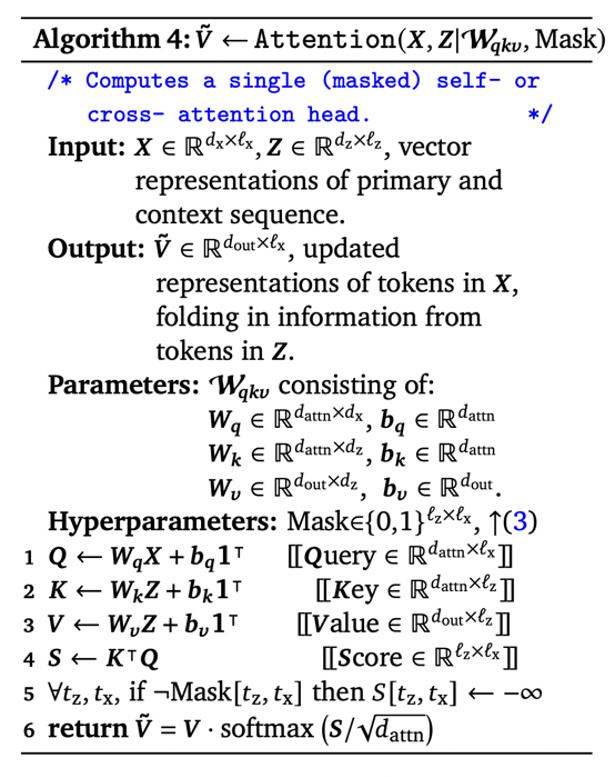
single query attention이 하나의 token에 대한 attention 과정이었다면 algorithm 4번의 attention은 이를 확장시켜 sequence에 존재하는 모든 token에 대해 attention을 진행하는 과정입니다.

Attention is All You Need에 소개된 $A(Q,K,V) = softmax(\frac{QK^T}{\sqrt{d_k}})V$을 그대로 적용합니다.

Input

• $X\in\R^{d_X \times l_X}$: primary sequence
• $Z\in\R^{d_Z \times l_Z}$: primary sequence에 대한 context sequence

Output

• $\tilde{V}\in\R^{d_{out} \times l_X}$: context 정보와 결합한 $X$에 존재하는 모든 token에 대한 vector represenations 반환
  • $\tilde{v} \in \R^{d_{out}}$
• 실제 Transformer에서는 attention 이후 residual connection을 하기 때문에 이 점에 유의해서 $d_{out}$과 $d_{in}$를 설정해주어야합니다.

Parameters

• $W_e \in \R^{d_{attn}\times d_{X}}$: query linear projection
  • $b_e \in \R^{d_{attn}}$: bias term
• $W_k \in \R^{d_{attn}\times d_{Z}}$: key linear projection
  • $b_k \in \R^{d_{attn}}$: bias term
• $W_v \in \R^{d_{out}\times d_{Z}}$: value linear projection
  • $b_v \in \R^{d_{out}}$: bias term

Hyperparameters

• $\text{Mask} \in \{0,1\}^{l_z \times l_x}$

과정

• 1~ 4번: single query attention에서 1 ~ 3번 과정을 행렬로 확장시킨 것입니다.
• 5번: 계산된 score에 mask를 사용하는 부분이 등장합니다.
  • mask값이 0인 부분에 아주 작은 값을 할당해서 softmax를 통과할 때 0에 가까운 값이 반환되도록 합니다.
• 6번: single query attention에서 4 ~5번 과정을 행렬로 확장시킨 것입니다.

self-attention

self-attention은 자기자신만을 사용하여 attention을 계산합니다. 따라서 $Z =X$인 Attention 입니다.

Bidirectional / unmasked self-attention

bidirectional / unmasked self-attention의 경우 sequence에 존재하는 모든 token에 대해 attention을 계산합니다. 따라서 $\text{Mask} \equiv 1$ 이면서 $Z=X$인 Attention입니다.

Unidirectional / masked self-attention

Unidirectional / masked self-attention의 경우 이전 token들을 context로 사용하여 각 token에 대해 attention을 계산합니다.

현재 token 다음에 나오는 token들은 maksed out되기 때문에 $\text{Mask} \coloneqq [[t_z \le t_x]]$이면서 $Z = X$인 Attention 입니다.

Cross-attention

primary sequence와 context sequence가 다른 attention입니다. self-attention에 반대되는 경우라고 볼 수 있기 때문에 $Z \ne X$입니다. cross-attention은 또한 mask를 적용하지 않기 때문에 $\text{mask} \equiv 1$인 Attention 입니다.

Algorithm 5: MHAttention

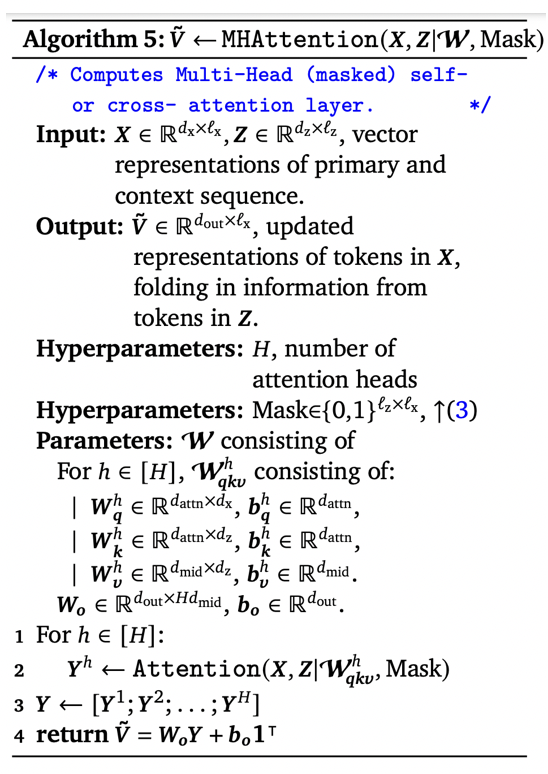
Input

• $X\in\R^{d_X \times l_X}$: primary sequence
• $Z\in\R^{d_Z \times l_Z}$: primary sequence에 대한 context sequence

Output

• $\tilde{V}\in\R^{d_{out} \times l_X}$: context 정보와 결합하여 $X$에 존재하는 모든 token에 대한 vector represenations 반환
  • $\tilde{v} \in \R^{d_{out}}$
• 실제 Transformer에서는 attention 이후 residual connection을 하기 때문에 이 점에 유의해서 $d_{out}$과 $d_{in}$를 설정해주어야합니다.

Parameters

• $H$: head 수
• $h \in [H]$에 대해서,
  • $W_e^h \in \R^{d_{attn}\times d_{X}}$: query linear projection
    • $b_e^h \in \R^{d_{attn}}$$b_e \in \R^{d_{attn}}$: bias term
  • $W_k^h \in \R^{d_{attn}\times d_{Z}}$: key linear projection
    • $b_k^h \in \R^{d_{attn}}$: bias term
  • $W_v^h \in \R^{d_{mid} \times d_{Z}}$: value linear projection
    • $b_v^h \in \R^{d_{mid}}$: bias term
• $W_o \in \R^{d_{out} \times Hd_{mid}}$
  • $b_o \in \R^{d_{out}}$

Hyperparameters

• $\text{Mask} \in \{0,1\}^{l_z \times l_x}$

과정

• 1 ~ 2번: Algorithm 4에 나오는 Attention을 $h$번 적용한다.
• 3번: h개의 attention output을 모두 concatenation한다.
• 4번: linear projection을 적용하여 $\R^{d_{out}}$ vector로 변환한다.

Algorithm 6. layer_norm

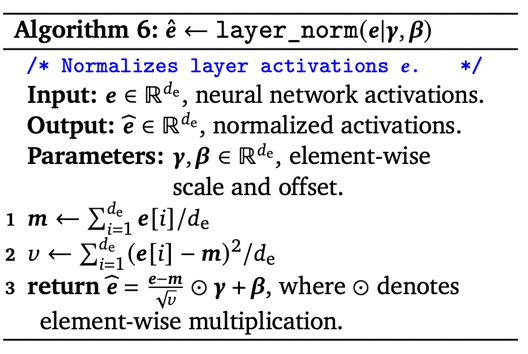
Input

• $e \in \R^{d_e}$: neural network activations
  • attention, position-wise feed forward의 output이 layer_norm의 input으로 들어갑니다.

Output

• $\hat{e} \in \R^{d_e}$: normalized activations

Parameters

• $\gamma, \beta \in \R^{d_e}$: element-wise scale($\gamma$)and offset($\beta$)

과정

• 1번: mean을 계산합니다.
• 2번: variance를 계산합니다.
• 3번: $e$를 standard normalization으로 바꾼 이후에 element-wise scaling과 offset을 적용해줍니다.
  • $\hat{e} \sim (0,1^2)$ → $\hat{e} \sim (0,\gamma^2)$ → $\hat{e} \sim (\beta,\gamma^2)$ 로 변화된다.
  • 데이터가 가지는 확률 분포를 학습하기 위해 standard normalization으로 바꾼 이후 mean, variance를 찾는 과정이라고 생각할 수 있다.

Algorithm 7. Unembedding

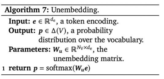
Input

• $e \in \R^{d_e}$: a token encoding
  • encoding된 token을 의미한다.

Output

• $p \in \Delta(V)$: a probability distibution over the vocabulary
  • vocabulary에 등장하는 token에 대한 확률을 의미한다.

Parameters

• $W_u \in \R^{N_V\times d_e}$: the embedding matrix

과정

• 1번: encoding된 token의 dimension을 $N_V$로 변환합니다. 이후 softmax를 이용해 vocabulary에서 각 token이 등장할 확률을 계산합니다.
  • $N_V$로 변환된 dimension의 각 index는 결국 vocabulary의 각 token들을 가리킵니다. 만약 softmax를 통과한 1번 index의 값이 0.9라면 1번 token이 등장할 확률이 0.9라는 뜻이 됩니다.

그 외

• Algorithm 1~7번을 바탕으로 Algorithm 8 ~ 15번에는Transformers 모델 구조, train 방법, inference 방법에 대한 pseudocode를 제시하고 있습니다.
  • Algorithm 8 ~ 15번에 소개되는 pseudocode에 대해서도 같이 살펴볼 수 있으면 좋겠습니다.
• Section 6번부터는 Encoder-Decoder, Encoder-only, Decoder-only Transformer에 대한 preview를 같이 제공하고 있습니다.
• Transformer를 이용하여 독일어를 영어로 번역하는 실습을 간단하게 여기서 해볼 수 있습니다.