Logistic Regression

로지스틱 회귀란, 회귀를 통해 나온 결과를 활성화 함수를 통해 확률로 변경하는 알고리즘이다.

이때 사용하는 회귀에 대한 개념은 다음 글에 정리했다. 선형회귀란?

로지스틱 함수는 독립변수 (-inf, inf) => (0,1)의 확률로 바꿔주는데 이때 알아야 할 개념이 오즈(odds)와 로짓(logit)이 있다.

• 오즈(odds)
  오즈는 사건이 발생할 확률을 사건이 발생하지 않을 확률로 나눠주는 것이다.

  odds = P(사건이 발생) / P(사건이 발생x)

• 로짓(logit)
  로짓은 이름에서도 볼 수 있다시피 오즈에 log를 씌워준 것이다.

  log를 씌워주는 이유는 입력값의 범위([0,1] - 확률이므로 0~1의 범위 값을 가짐)를 출력 시 (-inf, inf)로 바꿔주기 위함이다.

  logit = log(odds)

• 로지스틱 함수(sigmoid)
  로짓의 역함수로 종속변수가 1에 속할 확률을 나타내준다.

  logistic = $e^{x}/1+e^{x}$

보통 딥러닝이나 머신러닝에서는 로지스틱 함수(sigmoid)를 통해 나온 확률의 임계값(threshold)을 0.5로 설정하고 임계값이 넘으면 1로 아니면 0으로 리턴한다.

이때 loss 값은 다음과 같다. (y : label, h(x) : 회귀식)

loss function = -y*log(h(x)) - (1-y)*log(1-h(x))

간단한 텐서플로우 코드를 통해 로지스틱 회귀를 구현해보자.

# import
import numpy as np
import matplotlib.pyplot as plt
import tensorflow as tf

# data
np.random.seed(2022)
x1 = np.random.randint(1,10, size=10)
x2 = np.random.randint(1,5, size=(10))

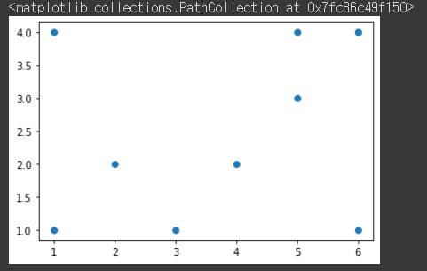
plt.scatter(x1,x2)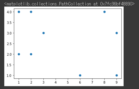

입력값 x_data의 분포는 위 그림과 같다. 이때 값이 y 축의 값이 2를 기준으로 분류를 해보자.

x_data = np.array([x1,x2]).T
y_data = [[1] if i>2 else [0] for i in x2]

all_data = np.hstack([x_data,y_data])
plt.scatter(all_data[:,:-2], all_data[:,-2:-1], c=all_data[:, 2])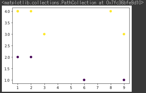

2 이상일 경우 노란색 미만일 경우 보라색으로 분류된 것을 확인할 수 있다.

그렇다면 학습을 통해 위 그림처럼 분류를 할 수 있도록 만들어 보자.

# dataset
dataset = tf.data.Dataset.from_tensor_slices((x_data, y_data)).batch(len(x_data))

# weight & bias
W = tf.Variable(tf.random.normal([2,1]))
b = tf.Variable(tf.random.normal([1]))

# loss function
def loss_fn(x, y):
  hypothesis = tf.math.sigmoid(tf.matmul(x,W) + b)
  loss = -y * tf.math.log(hypothesis) - (1-y) * tf.math.log(1-hypothesis)
  loss = tf.reduce_mean(loss)
  return loss

# gradients
def grad(x, y):
  with tf.GradientTape() as tape:
    loss = loss_fn(x,y)
    return tape.gradient(loss, [W,b])

# optimizer
optimizer = tf.keras.optimizers.SGD(learning_rate=3e-2) # Adam이나 다른 옵티마이저도 사용 가능

epochs = 2000
lr = 1e-3

for epoch in range(1, epochs+1):
  for x, y in dataset:
    grads = grad(x,y)
    optimizer.apply_gradients(grads_and_vars=zip(grads, [W,b]))  
    if epoch % 200 == 0:
      print("Epoch : {:2}, Loss : {:4f}".format(epoch, loss_fn(x,y)))
    

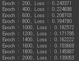
총 2,000번 학습을 했고 이 모델은 과적합이 됐을 것이다. 하지만 이번에는 테스트 데이터 없이 분류를 할 수 있는지에만 초점을 맞췄기 때문에 신경쓰지 않겠다.

# predict
prediction = tf.cast(tf.sigmoid(tf.matmul(x_data,W)+b)>0.5, dtype=tf.float32)
acc = tf.reduce_mean(tf.cast(tf.equal(prediction, y_data),dtype=tf.float32))
print("Accuracy : {:.2f}%".format(acc*100))

예측된 y값과 실제값 y가 전부 일치한 것을 확인할 수 있다.