Non-linear Least Squares
Introduction
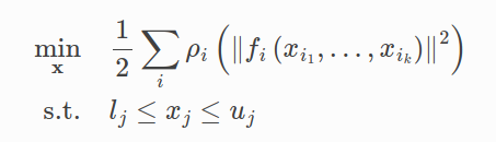
Ceres-Solver를 이용하면 아래와 같은 bounds constrained robustified non-linear least squares problem을 풀 수 있다.
ResidualBlock :
CostFunction : that depends on the parameter blocks.
ParameterBlock :
LossFunction : . non-linear least squares problem을 해결하는 데 outlier의 영향을 줄이는 역할을 한다.
Hello World!
간단히 의 solution을 ceres-solver를 이용해 구해보자.
CostFunction :
ParameterBlock :
LossFunction :
먼저 CostFunction에 대한 CostFunctor를 작성해야 한다.
중요한 점은 operator()는 templated method이기 때문에 Ceres는
CostFunctor::operator<T>()와 같이 호출할 수 있다.
residual의 value가 필요한 경우에는 T=double, Jacobians이 필요한 경우에는 T=Jet을 사용.
code
#include <iostream>

#include <ceres/ceres.h>

struct CostFunctor
{
    template <typename T>
    bool operator()(const T* const x, T* residual) const
    {
        residual[0] = 10.0 - x[0];
        return true;
    }
};


int main(int argc, char** argv)
{
    double initialX = 5.0;
    double x = initialX;

    ceres::Problem problem;

    // This uses auto-diff to obtain the derivative(jacobian)
    ceres::CostFunction* costFunction = new ceres::AutoDiffCostFunction<CostFunctor, 1, 1>(new CostFunctor);
    problem.AddResidualBlock(costFunction, nullptr, &x);

    ceres::Solver::Options options;
    options.linear_solver_type = ceres::DENSE_QR;
    options.minimizer_progress_to_stdout = true;
    ceres::Solver::Summary summary;
    ceres::Solve(options, &problem, &summary);

    std::cout << summary.BriefReport() << "\n";
    std::cout << "x : " << initialX << " -> " << x << "\n";
}
result
iter      cost      cost_change  |gradient|   |step|    tr_ratio  tr_radius  ls_iter  iter_time  total_time
   0  1.250000e+01    0.00e+00    5.00e+00   0.00e+00   0.00e+00  1.00e+04        0    1.31e-05    3.41e-05
   1  1.249750e-07    1.25e+01    5.00e-04   0.00e+00   1.00e+00  3.00e+04        1    2.50e-05    3.94e-04
   2  1.388518e-16    1.25e-07    1.67e-08   5.00e-04   1.00e+00  9.00e+04        1    3.81e-06    4.02e-04
Ceres Solver Report: Iterations: 3, Initial cost: 1.250000e+01, Final cost: 1.388518e-16, Termination: CONVERGENCE
x : 5 -> 10
Derivatives
다른 optimization package들과 마찬가지로 ceres 또한 objective function의 각 term들에 대한 값과 derivatives를 알 수 있다. ceres는 몇몇 방법들을 제공하는데 위에서 사용한 auto-diff 이외에 Analytic, numeric derivatives에 대해 살펴보자.
Numeric Derivatives
종종 templated cost functor를 정의하는 것이 불가능하다. 예를 들어 residual을 계산하는 데 특정한 라이브러리의 함수를 호출하는 경우이다. 이 때, numeric differentiation을 사용할 수 있다. 사용자는 residual value를 계산하는 functor를 정의하고, NumericDiffCostFunctor를 사용한다.
struct NumericDiffCostFunctor
{
    bool operator()(const double* const x, double* residual) const
    {
        residual[0] = 10.0 - x[0];
        return true;
    }
};

int main(int argc, char** argv)
{
    double initialX = 5.0;
    double x = initialX;

    ceres::Problem problem;

    // This uses auto-diff to obtain the derivative(jacobian)
    ceres::CostFunction* costFunction = new ceres::NumericDiffCostFunction<NumericDiffCostFunctor, 	ceres::CENTRAL, 1, 1>(new NumericDiffCostFunctor);
    problem.AddResidualBlock(costFunction, nullptr, &x);

    ceres::Solver::Options options;
    options.linear_solver_type = ceres::DENSE_QR;
    options.minimizer_progress_to_stdout = true;
    ceres::Solver::Summary summary;
    ceres::Solve(options, &problem, &summary);

    std::cout << summary.BriefReport() << "\n";
    std::cout << "x : " << initialX << " -> " << x << "\n";
}
일반적으로 auto-diff를 추천한다. 그 이유는 C++ templates를 사용하면 auto-diff가 효율적이게 되기 때문이다.
Analytic Derivatives
종종 auto-diff를 사용하는 것이 불가능한 경우가 있다. 예를 들어 auto-diff가 chain rule을 이용해 계산하는 것보다 analytic한 방법으로 closed form으로 derivatives를 구하는 게 더 효율적인 경우이다.
그러한 경우에, 사용자의 residual과 jacobian computation code를 제공하는 것이 가능하다.
그러기 위해서는 CostFunction 또는 SizedCostFunction의 subclass 를 정의해야 한다. SizedCostFunction는 parameters와 residual의 size를 compile time에 알고있을 경우에 사용한다.
아래는 에 대한 예시이다.
class QuadraticCostFunction : public ceres::SizedCostFunction<1, 1>
{
public:
    virtual ~QuadraticCostFunction()
    {
    }
    virtual bool Evaluate(double const *const *parameters, double *residuals, double **jacobians) const
    {
        const double x = parameters[0][0];
        residuals[0] = 10.0 - x;

        //  compute jacobian if asked for
        if (jacobians != nullptr && jacobians[0] != nullptr)
        {
            jacobians[0][0] = -1;
        }
        return true;
    }

private:
};
확실한 이유가 있는 게 아니라면 analytic 보다는 autodiff, numericdiff를 더 추천한다.
More About Derivatives
이외에도 DynamicAutoDiffCostFunction, CostFunctionToFunctor, NumericDiffFunctor, ConditionedCostFunction이 존재한다.
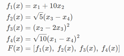
Powell's Function
minimization of Powell's Function 문제를 해결해보자.
CostFunction :
ParameterBlock :
LossFunction :
4개의 costFunctor를 정의한 뒤에 AddResidualBlock을 이용해 추가해준다.
code
#include <iostream>

#include <ceres/ceres.h>

struct F1
{
    template <typename T>
    bool operator()(const T *const x1, const T *const x2, T *residual) const
    {
        residual[0] = x1[0] + 10.0 * x2[0];
        return true;
    }
};

struct F2
{
    template <typename T>
    bool operator()(const T *const x3, const T *const x4, T *residual) const
    {
        residual[0] = std::sqrt(5.0) * (x3[0] - x4[0]);
        return true;
    }
};

struct F3
{
    template <typename T>
    bool operator()(const T *const x2, const T *const x3, T *residual) const
    {
        residual[0] = (x2[0] - 2.0 * x3[0]) * (x2[0] - 2.0 * x3[0]);
        return true;
    }
};

struct F4
{
    template <typename T>
    bool operator()(const T *const x1, const T *const x4, T *residual) const
    {
        residual[0] = std::sqrt(10.0) * (x1[0] - x4[0]) * (x1[0] - x4[0]);
        return true;
    }
};

int main()
{
    double x1(-3.0), x2(-1.0), x3(0.0), x4(1.0);

    ceres::Problem problem;

    // This uses auto-diff to obtain the derivative(jacobian)

    problem.AddResidualBlock(new ceres::AutoDiffCostFunction<F1, 1, 1, 1>(new F1), nullptr, &x1, &x2);
    problem.AddResidualBlock(new ceres::AutoDiffCostFunction<F2, 1, 1, 1>(new F2), nullptr, &x3, &x4);
    problem.AddResidualBlock(new ceres::AutoDiffCostFunction<F3, 1, 1, 1>(new F3), nullptr, &x2, &x3);
    problem.AddResidualBlock(new ceres::AutoDiffCostFunction<F4, 1, 1, 1>(new F4), nullptr, &x1, &x4);

    ceres::Solver::Options options;

    options.max_num_iterations = 100;
    options.linear_solver_type = ceres::DENSE_QR;
    options.minimizer_progress_to_stdout = true;
    ceres::Solver::Summary summary;
    ceres::Solve(options, &problem, &summary);

    std::cout << summary.FullReport() << "\n";

    std::cout << "solution x1 : " << x1 << ", x2 : " << x2 << ", x3 : " << x3 << ", x4 : " << x4 << "\n";

    return 0;
}
result
iter      cost      cost_change  |gradient|   |step|    tr_ratio  tr_radius  ls_iter  iter_time  total_time
   0  1.367500e+03    0.00e+00    1.29e+03   0.00e+00   0.00e+00  1.00e+04        0    9.51e-05    1.78e-04
   1  8.005063e+01    1.29e+03    1.60e+02   0.00e+00   9.41e-01  3.00e+04        1    1.49e-04    4.26e-04
   2  5.003649e+00    7.50e+01    2.00e+01   8.76e-01   9.37e-01  9.00e+04        1    6.82e-05    5.17e-04
   3  3.127387e-01    4.69e+00    2.50e+00   4.36e-01   9.37e-01  2.70e+05        1    6.10e-05    5.94e-04
   4  1.954643e-02    2.93e-01    3.13e-01   2.18e-01   9.37e-01  8.10e+05        1    6.01e-05    6.68e-04
   5  1.221660e-03    1.83e-02    3.91e-02   1.09e-01   9.37e-01  2.43e+06        1    5.89e-05    7.41e-04
   6  7.635418e-05    1.15e-03    4.88e-03   5.45e-02   9.37e-01  7.29e+06        1    5.79e-05    8.14e-04
   7  4.772166e-06    7.16e-05    6.11e-04   2.72e-02   9.37e-01  2.19e+07        1    6.01e-05    8.88e-04
   8  2.982627e-07    4.47e-06    7.63e-05   1.36e-02   9.37e-01  6.56e+07        1    5.98e-05    9.63e-04
   9  1.864162e-08    2.80e-07    9.54e-06   6.81e-03   9.37e-01  1.97e+08        1    6.10e-05    1.05e-03
  10  1.165117e-09    1.75e-08    1.19e-06   3.40e-03   9.37e-01  5.90e+08        1    5.91e-05    1.12e-03
  11  7.282117e-11    1.09e-09    1.49e-07   1.70e-03   9.37e-01  1.77e+09        1    6.08e-05    1.19e-03
  12  4.551435e-12    6.83e-11    1.86e-08   8.51e-04   9.37e-01  5.31e+09        1    6.01e-05    1.27e-03
  13  2.844741e-13    4.27e-12    2.33e-09   4.26e-04   9.37e-01  1.59e+10        1    6.01e-05    1.35e-03
  14  1.778041e-14    2.67e-13    2.91e-10   2.13e-04   9.37e-01  4.78e+10        1    6.01e-05    1.42e-03
  15  1.111340e-15    1.67e-14    3.64e-11   1.06e-04   9.37e-01  1.43e+11        1    5.98e-05    1.49e-03

Solver Summary (v 2.2.0-eigen-(3.3.7)-lapack-suitesparse-(5.7.1)-eigensparse)

                                     Original                  Reduced
Parameter blocks                            4                        4
Parameters                                  4                        4
Residual blocks                             4                        4
Residuals                                   4                        4

Minimizer                        TRUST_REGION

Dense linear algebra library            EIGEN
Trust region strategy     LEVENBERG_MARQUARDT
                                        Given                     Used
Linear solver                        DENSE_QR                 DENSE_QR
Threads                                     1                        1
Linear solver ordering              AUTOMATIC                        4

Cost:
Initial                          1.367500e+03
Final                            1.111340e-15
Change                           1.367500e+03

Minimizer iterations                       16
Successful steps                           16
Unsuccessful steps                          0

Time (in seconds):
Preprocessor                         0.000083

  Residual only evaluation           0.000027 (15)
  Jacobian & residual evaluation     0.000863 (16)
  Linear solver                      0.000093 (15)
Minimizer                            0.001433

Postprocessor                        0.000007
Total                                0.001523

Termination:                      CONVERGENCE (Gradient tolerance reached. Gradient max norm: 3.639531e-11 <= 1.000000e-10)

solution x1 : -0.000102043, x2 : 1.02043e-05, x3 : 2.00475e-05, x4 : 2.00475e-05
Curve Fitting
지금까지의 예제들은 data가 없는 간단한 optimization 문제들이었다. least squares, non-linear least squares의 본래 목적은 data의 curve fitting이었다.
이번에는 curve로부터 sample을 뽑고, standard deviation 의 가우시안 노이즈를 더한 뒤 의 curve fitting을 수행할 것이다.
code
#include <iostream>
#include <random>

#include <ceres/ceres.h>

struct ExponentialResidual
{
    ExponentialResidual(double x, double y)
        : x_(x), y_(y)
    {
    }

    template <typename T>
    bool operator()(const T *const m, const T *const c, T *residual) const
    {
        residual[0] = y_ - exp(m[0] * x_ + c[0]);
        return true;
    }

private:
    const double x_;
    const double y_;
};

int main()
{
    const int kNumObservations = 67;

    double data[kNumObservations * 2];

    std::mt19937 gen(23497);
    std::normal_distribution<double> dist(0.0, 0.2);
    for (int i = 0; i < kNumObservations; ++i)
    {
        double x = 0.075 * static_cast<double>(i);
        double y = exp(0.3 * x + 0.1);

        data[2*i] = x;
        data[2*i + 1] = y + dist(gen);
    }

    double m(0.0), c(0.0); // y = e^(mx+c)

    ceres::Problem problem;
    for (int i = 0; i < kNumObservations; ++i)
    {
        ceres::CostFunction *costFunction = new ceres::AutoDiffCostFunction<ExponentialResidual, 1, 1, 1>(new ExponentialResidual(data[2 * i], data[2 * i + 1]));
        problem.AddResidualBlock(costFunction, nullptr, &m, &c);
    }

    ceres::Solver::Options options;

    options.max_num_iterations = 25;
    options.linear_solver_type = ceres::DENSE_QR;
    options.minimizer_progress_to_stdout = true;
    ceres::Solver::Summary summary;
    ceres::Solve(options, &problem, &summary);

    std::cout << summary.BriefReport() << "\n";
    std::cout << "Final m : " << m << ", c : " << c << "\n";
    return 0;
}
result
iter      cost      cost_change  |gradient|   |step|    tr_ratio  tr_radius  ls_iter  iter_time  total_time
   0  1.224747e+02    0.00e+00    3.62e+02   0.00e+00   0.00e+00  1.00e+04        0    1.94e-04    2.30e-04
   1  2.574039e+03   -2.45e+03    3.62e+02   0.00e+00  -2.05e+01  5.00e+03        1    3.50e-05    2.81e-04
   2  2.570054e+03   -2.45e+03    3.62e+02   0.00e+00  -2.05e+01  1.25e+03        1    5.01e-06    2.90e-04
   3  2.546365e+03   -2.42e+03    3.62e+02   0.00e+00  -2.03e+01  1.56e+02        1    4.05e-06    2.99e-04
   4  2.342206e+03   -2.22e+03    3.62e+02   0.00e+00  -1.86e+01  9.77e+00        1    7.87e-06    3.11e-04
   5  8.885636e+02   -7.66e+02    3.62e+02   0.00e+00  -6.56e+00  3.05e-01        1    4.05e-06    3.29e-04
   6  3.493132e+01    8.75e+01    4.15e+02   0.00e+00   1.37e+00  9.16e-01        1    2.09e-04    5.41e-04
   7  7.793141e+00    2.71e+01    1.87e+02   1.27e-01   1.11e+00  2.75e+00        1    1.85e-04    7.29e-04
   8  4.377171e+00    3.42e+00    5.98e+01   3.56e-02   1.03e+00  8.24e+00        1    1.83e-04    9.15e-04
   9  2.676740e+00    1.70e+00    2.62e+01   1.00e-01   9.90e-01  2.47e+01        1    1.86e-04    1.10e-03
  10  1.694918e+00    9.82e-01    9.22e+00   1.19e-01   9.84e-01  7.42e+01        1    1.83e-04    1.29e-03
  11  1.503587e+00    1.91e-01    1.55e+00   7.01e-02   9.91e-01  2.22e+02        1    1.82e-04    1.48e-03
  12  1.495106e+00    8.48e-03    1.10e-01   1.73e-02   9.93e-01  6.67e+02        1    1.78e-04    1.66e-03
  13  1.495053e+00    5.29e-05    2.03e-03   1.45e-03   9.93e-01  2.00e+03        1    1.77e-04    1.84e-03
Ceres Solver Report: Iterations: 14, Initial cost: 1.224747e+02, Final cost: 1.495053e+00, Termination: CONVERGENCE
Final m : 0.306178, c : 0.0788425
m=0.3, c=0.1을 이용해 sampling을 했는데 solver를 통해 구한 c = 0.0788425로 약간 부정확하다. 이것은 예견된 결과이다. noisy한 data로부터 curve fitting을 수행하면 이러한 deviation이 생길 수 밖에 없다.
Robust Curve Fitting
outlier에 대응하기 위해 standard technique로 LossFunction이 있다.
LossFunction은 residual 값이 아주 큰 residual block들의 영향을 줄여준다.
위 코드를 다음과 같이 수정해서 CauchyLoss를 사용할 수 있다.
problem.AddResidualBlock(cost_function, new CauchyLoss(0.5) , &m, &c);
result
iter      cost      cost_change  |gradient|   |step|    tr_ratio  tr_radius  ls_iter  iter_time  total_time
   0  1.711812e+01    0.00e+00    2.06e+01   0.00e+00   0.00e+00  1.00e+04        0    1.99e-04    2.24e-04
   1  2.174156e+01   -4.62e+00    2.06e+01   0.00e+00  -8.35e-01  5.00e+03        1    1.81e-05    2.69e-04
   2  2.173498e+01   -4.62e+00    2.06e+01   0.00e+00  -8.34e-01  1.25e+03        1    5.01e-06    2.78e-04
   3  2.169558e+01   -4.58e+00    2.06e+01   0.00e+00  -8.26e-01  1.56e+02        1    5.01e-06    2.86e-04
   4  2.133292e+01   -4.21e+00    2.06e+01   0.00e+00  -7.61e-01  9.77e+00        1    5.01e-06    2.94e-04
   5  1.611761e+01    1.00e+00    8.39e+01   0.00e+00   1.85e-01  7.81e+00        1    1.86e-04    4.82e-04
   6  6.829044e+00    9.29e+00    1.09e+02   9.28e-02   2.07e+00  2.34e+01        1    1.84e-04    6.69e-04
   7  2.031437e+00    4.80e+00    7.42e+01   6.89e-02   1.81e+00  7.03e+01        1    1.98e-04    8.70e-04
   8  1.300223e+00    7.31e-01    1.92e+01   5.60e-02   1.29e+00  2.11e+02        1    1.87e-04    1.06e-03
   9  1.242393e+00    5.78e-02    3.47e+00   3.09e-02   1.18e+00  6.32e+02        1    1.95e-04    1.26e-03
  10  1.238930e+00    3.46e-03    5.23e-01   9.85e-03   1.19e+00  1.90e+03        1    1.98e-04    1.46e-03
  11  1.238756e+00    1.74e-04    6.70e-02   2.47e-03   1.21e+00  5.69e+03        1    1.85e-04    1.65e-03
  12  1.238747e+00    8.55e-06    6.31e-03   5.75e-04   1.22e+00  1.71e+04        1    1.90e-04    1.84e-03
Ceres Solver Report: Iterations: 13, Initial cost: 1.711812e+01, Final cost: 1.238747e+00, Termination: CONVERGENCE
Final m : 0.305461, c : 0.0820266
Bundle Adjustment
Ceres가 작성된 가장 큰 이유들 중 하나는 large scale bundle adjustment 문제를 풀기 위해서였다.
image feature의 locations와 correspondences가 주어졌을 때, BA의 목표는 reprojection error를 최소화하는 3D point position과 camera parameters를 찾는 것이다.
BAL dataset을 이용해 실습을 진행한다.
우선 reprojection error/residual을 계산하는 templated functor를 정의한다. residual은 camera의 9개 파라미터와 point의 3개 파라미터에 대한 함수이다.
camera에는 3개의 axis-angle vector, 3개의 translation vector, 1개의 focal length, 2개의 radial distortion coefficient가 들어있다.
"ceres/rotation.h"의 AngleaxisRotatePoint()함수르 이용해 3D point를 회전시킬 수 있다.
linear_solver_type은 sparse한 성질을 활용해 SPARSE_NORMAL_CHOLESKY를 사용해볼 수 있다. 하지만 BA 문제는 더 효율적으로 계산 가능한 구조를 가지고 있기 때문에 Schure 기반 솔버를 사용하는것이 좋다. Ceres는 총 3개의 슈어 기반 솔버를 제공하고 그 중 가장 간단한 DENSE_SCHUR를 사용한다.
result
50 iter 후에도 수렴하지 않아 강제종료 되었다.
iter      cost      cost_change  |gradient|   |step|    tr_ratio  tr_radius  ls_iter  iter_time  total_time
   0  1.115206e+07    0.00e+00    8.66e+07   0.00e+00   0.00e+00  1.00e+04        0    1.46e+01    1.49e+01
   1  9.460718e+05    1.02e+07    4.51e+07   0.00e+00   9.53e-01  3.00e+04        1    1.48e+01    2.97e+01
   2  1.505154e+07   -1.41e+07    4.51e+07   7.84e+02  -2.10e+01  1.50e+04        1    2.38e-01    2.99e+01
   3  5.127748e+05    4.33e+05    8.06e+06   4.98e+02   6.55e-01  1.55e+04        1    1.48e+01    4.47e+01
   4  8.860289e+05   -3.73e+05    8.06e+06   3.82e+02  -1.52e+00  7.73e+03        1    2.38e-01    4.49e+01
   5  1.611821e+06   -1.10e+06    8.06e+06   2.06e+02  -4.53e+00  1.93e+03        1    2.32e-01    4.52e+01
   6  3.156876e+05    1.97e+05    5.36e+05   5.74e+01   8.41e-01  2.83e+03        1    1.48e+01    6.00e+01
   7  2.804119e+05    3.53e+04    1.91e+05   8.32e+01   8.00e-01  3.61e+03        1    1.48e+01    7.47e+01
   8  2.671542e+05    1.33e+04    1.21e+05   1.06e+02   9.13e-01  8.27e+03        1    1.49e+01    8.97e+01
   9  2.983934e+05   -3.12e+04    1.21e+05   2.25e+02  -3.05e+00  4.14e+03        1    2.78e-01    9.00e+01
  10  2.601057e+05    7.05e+03    2.33e+05   1.23e+02   9.50e-01  1.24e+04        1    1.51e+01    1.05e+02
  11  2.545691e+05    5.54e+03    8.40e+05   3.17e+02   8.03e-01  1.60e+04        1    1.50e+01    1.20e+02
  12  2.514598e+05    3.11e+03    1.13e+06   3.95e+02   8.25e-01  2.20e+04        1    1.49e+01    1.35e+02
  13  2.497169e+05    1.74e+03    1.54e+06   5.32e+02   7.72e-01  2.63e+04        1    1.49e+01    1.50e+02
  14  2.483271e+05    1.39e+03    1.59e+06   6.23e+02   7.66e-01  3.09e+04        1    1.49e+01    1.65e+02
  15  2.471678e+05    1.16e+03    1.50e+06   7.17e+02   7.59e-01  3.59e+04        1    1.51e+01    1.80e+02
  16  2.462096e+05    9.58e+02    1.38e+06   8.13e+02   7.55e-01  4.14e+04        1    1.48e+01    1.95e+02
  17  2.454271e+05    7.82e+02    1.25e+06   9.15e+02   7.52e-01  4.75e+04        1    1.48e+01    2.09e+02
  18  2.447916e+05    6.35e+02    1.13e+06   1.02e+03   7.50e-01  5.43e+04        1    1.48e+01    2.24e+02
  19  2.442756e+05    5.16e+02    1.03e+06   1.14e+03   7.48e-01  6.18e+04        1    1.50e+01    2.39e+02
  20  2.438554e+05    4.20e+02    9.51e+05   1.27e+03   7.46e-01  7.01e+04        1    1.52e+01    2.54e+02
  21  2.435118e+05    3.44e+02    8.85e+05   1.42e+03   7.44e-01  7.93e+04        1    1.52e+01    2.70e+02
  22  2.432296e+05    2.82e+02    8.29e+05   1.59e+03   7.41e-01  8.93e+04        1    1.49e+01    2.85e+02
  23  2.429968e+05    2.33e+02    7.78e+05   1.79e+03   7.39e-01  1.00e+05        1    1.50e+01    3.00e+02
  24  2.428042e+05    1.93e+02    7.31e+05   2.02e+03   7.36e-01  1.12e+05        1    1.49e+01    3.14e+02
  25  2.426440e+05    1.60e+02    6.85e+05   2.37e+03   7.35e-01  1.25e+05        1    1.48e+01    3.29e+02
  26  2.425104e+05    1.34e+02    6.36e+05   2.88e+03   7.35e-01  1.39e+05        1    1.49e+01    3.44e+02
  27  2.423987e+05    1.12e+02    5.81e+05   3.59e+03   7.39e-01  1.57e+05        1    1.51e+01    3.59e+02
  28  2.423059e+05    9.28e+01    5.16e+05   4.50e+03   7.50e-01  1.79e+05        1    1.51e+01    3.74e+02
  29  2.422300e+05    7.58e+01    4.42e+05   5.41e+03   7.65e-01  2.10e+05        1    1.49e+01    3.89e+02
  30  2.421694e+05    6.07e+01    3.70e+05   6.31e+03   7.81e-01  2.56e+05        1    1.49e+01    4.04e+02
  31  2.421213e+05    4.81e+01    3.06e+05   7.17e+03   7.95e-01  3.22e+05        1    1.50e+01    4.19e+02
  32  2.420828e+05    3.85e+01    2.54e+05   8.06e+03   8.08e-01  4.21e+05        1    1.51e+01    4.34e+02
  33  2.420512e+05    3.16e+01    2.12e+05   9.11e+03   8.20e-01  5.70e+05        1    1.49e+01    4.49e+02
  34  2.420243e+05    2.69e+01    1.80e+05   1.04e+04   8.30e-01  7.99e+05        1    1.50e+01    4.64e+02
  35  2.420005e+05    2.38e+01    1.57e+05   1.22e+04   8.38e-01  1.15e+06        1    1.48e+01    4.79e+02
  36  2.419787e+05    2.18e+01    1.40e+05   1.45e+04   8.43e-01  1.71e+06        1    1.48e+01    4.94e+02
  37  2.419584e+05    2.04e+01    1.29e+05   1.74e+04   8.47e-01  2.57e+06        1    1.48e+01    5.09e+02
  38  2.419391e+05    1.93e+01    1.22e+05   2.10e+04   8.49e-01  3.88e+06        1    1.50e+01    5.24e+02
  39  2.419207e+05    1.83e+01    1.19e+05   2.54e+04   8.49e-01  5.88e+06        1    1.51e+01    5.39e+02
  40  2.419034e+05    1.74e+01    1.17e+05   3.05e+04   8.48e-01  8.86e+06        1    1.49e+01    5.54e+02
  41  2.418871e+05    1.63e+01    1.17e+05   3.65e+04   8.46e-01  1.32e+07        1    1.49e+01    5.68e+02
  42  2.418718e+05    1.52e+01    1.17e+05   4.32e+04   8.44e-01  1.96e+07        1    1.49e+01    5.83e+02
  43  2.418576e+05    1.42e+01    1.18e+05   5.09e+04   8.41e-01  2.87e+07        1    1.49e+01    5.98e+02
  44  2.418443e+05    1.33e+01    1.20e+05   5.94e+04   8.38e-01  4.16e+07        1    1.49e+01    6.13e+02
  45  2.418320e+05    1.23e+01    1.22e+05   6.89e+04   8.34e-01  5.92e+07        1    1.49e+01    6.28e+02
  46  2.418207e+05    1.14e+01    1.25e+05   7.89e+04   8.29e-01  8.29e+07        1    1.49e+01    6.43e+02
  47  2.418102e+05    1.05e+01    1.28e+05   8.96e+04   8.23e-01  1.14e+08        1    1.49e+01    6.58e+02
  48  2.418006e+05    9.61e+00    1.30e+05   1.00e+05   8.17e-01  1.53e+08        1    1.50e+01    6.73e+02
  49  2.417918e+05    8.79e+00    1.33e+05   1.11e+05   8.10e-01  2.00e+08        1    1.49e+01    6.88e+02
  50  2.417838e+05    8.02e+00    1.35e+05   1.21e+05   8.03e-01  2.58e+08        1    1.49e+01    7.03e+02

Solver Summary (v 2.2.0-eigen-(3.3.7)-lapack-suitesparse-(5.7.1)-eigensparse)

                                     Original                  Reduced
Parameter blocks                        64105                    64105
Parameters                             192627                   192627
Residual blocks                        347173                   347173
Residuals                              694346                   694346

Minimizer                        TRUST_REGION

Dense linear algebra library            EIGEN
Trust region strategy     LEVENBERG_MARQUARDT
                                        Given                     Used
Linear solver                     DENSE_SCHUR              DENSE_SCHUR
Threads                                     1                        1
Linear solver ordering              AUTOMATIC                 64053,52
Schur structure                         2,3,9                    2,3,9

Cost:
Initial                          1.115206e+07
Final                            2.417838e+05
Change                           1.091028e+07

Minimizer iterations                       51
Successful steps                           47
Unsuccessful steps                          4

Time (in seconds):
Preprocessor                         0.311499

  Residual only evaluation           2.474714 (50)
  Jacobian & residual evaluation   689.610311 (47)
  Linear solver                      8.894256 (50)
Minimizer                          702.245928

Postprocessor                        0.010002
Total                              702.567430

Termination:                   NO_CONVERGENCE (Maximum number of iterations reached. Number of iterations: 50.)