Outlier Detection with Autoencoder Ensembles
Outlier Detection with Autoencoder Ensembles
- 2017 SIAM International Conference on Data Mining (SDM)
Introduction
In this paper, authors proposed autoencoder ensemble method
: Randomized Neural Network for Outlier Detection(RandNet)
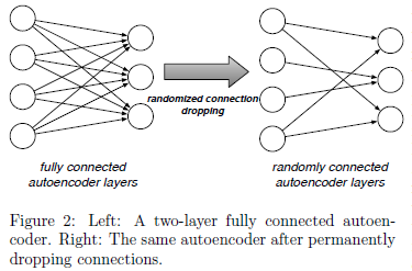
fully connected autoencoder 대신 randomly connected autoencoder를 사용
각 autoencoder는 structures와 connection densities가 서로 다름
➜ computational complexity ↓
Deep Neural Network의 overfitting 위험성이 존재하며 종종 local optima로 수렴
➜ 일부 structure가 overfit 되더라도 emsemble의 특성인 다양성으로 인하여 전반적으로 효율성이 향상될 수 있음
RandNet
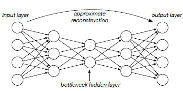
Autoencoder based model
➜ input과 output이 최대한 비슷하게 reconstruction하도록 model training
➜ latent vector는 input의 주요한 특성을 포함하고 있을 것
➜ anomaly는 잘 reconstruction x
fully connected auto-encoder example
train data에 anomaly가 포함되어 있는 경우가 많아 neural networks based methods 학습 시에 overfitting의 가능성이 높아짐
➜ overfitting의 문제 해결하기 위해 ensemble method 적용
but multiple methods의 조합이 항상 best performance를 보이는 individual model보다 더 나은 결과를 보인다고 보장할 수는 없음
따라서, ensemble method가 잘 작동하기 위해서는 각 구성 요소가 충분히 다양해야 함
다양한 구조가 조합되면 서로 다른 패턴을 포착하기 용이할 것
본 논문에서는 fully connected autoencoder를 사용하면 각 model의 output이 비슷할 것이기 때문에 randomly connected autoencoder를 사용
randomly connected auto-encoder example
RandNet과 dropout의 차이점
- RandNet : 서로 다른 구조의 NN model의 결과가 합쳐짐 ➜ 단일 구조의 overfitting의 큰 문제 없음
- Dropout : 단일 모델 내의 random connection ➜ overfitting 방지 목적
Neural Network Structure
autoencoder structure
각 layer에서 사용되는 node 수는 이전 layer의 node의 비율로 설정되며 최소 node 수는 3
➜ botteleck hidden layer에서 과도한 압축으로 인하여 발생하는 정보 손실을 막기 위해
Activation Function
첫 번째 hidden layer와 output layer : Sigmoid function
나머지 layer : ReLU
두 activation function의 장/단점의 균형을 맞추는 것을 목표로 하며,
해당 activation function 조합을 사용하였을 때 가장 좋은 성능을 보임
Anomaly score
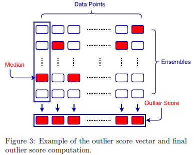
notation
- : the number of data points
- : data dimension
- : ensemble components
: -th ensemble component's -th input data point
: autoencoder's reconstructed output
data point의 final anomaly score는 ensemble의 median score로 계산
Conclusions
In this paper ...
- autoencoder ensemble
- adaptive data sampling
: training iteration에 따라 sampling size를 증가시키며 학습
