
1. 학습내용
Cutout (2017)
좋은 점 : 똑같은 이미지가 들어와도 정사각형 영역이 랜덤으로 가려져서 다른 이미지로 인식한다.
base라인이 96으로 되어있는데 cutout을 했을 때 성능이 상승한 것을 볼 수 있다.
성능 상승폭이 많이 크지는 않다 (0.5~0.8, 데이터가 조금 늘어나서 성능이 상승한 것)
albumentations 라이브러리에서 cutout을 제공하고 있다
import albumentations as A
import cv2
from torch.utils.data import Dataset
from albumentations.pytorch import ToTensorV2
from matplotlib import pyplot as plt
from torchvision import transforms


class AlbumentationsDataset(Dataset):

    def __init__(self, file_path, labels, transform=None):
        self.file_path = file_path
        self.labels = labels
        self.transform = transform

    def __getitem__(self, index):
        label = self.labels[index]
        file_path = self.file_path[index]

        image = cv2.imread(file_path)
        image = cv2.cvtColor(image, cv2.COLOR_BGR2RGB)

        if self.transform:
            augmented = self.transform(image = image)
            image = augmented['image']

        return image, label

    def __len__(self):
        return len(self.file_path)


albumentations_transform  = A.Compose([
    A.Resize(256, 256),
    A.RandomCrop(224, 224),
    A.Cutout(num_holes = 8, max_h_size = 30, max_w_size = 30, p = 1.0), #
    ToTensorV2()
])

albumentations_dataset = AlbumentationsDataset(
    file_path=["./image/orange.jpg"],
    labels = [1],
    transform = albumentations_transform
)

for i in range(100):
    sample, _ = albumentations_dataset[0]

plt.figure(figsize=(10, 10))
plt.imshow(transforms.ToPILImage()(sample))
plt.show()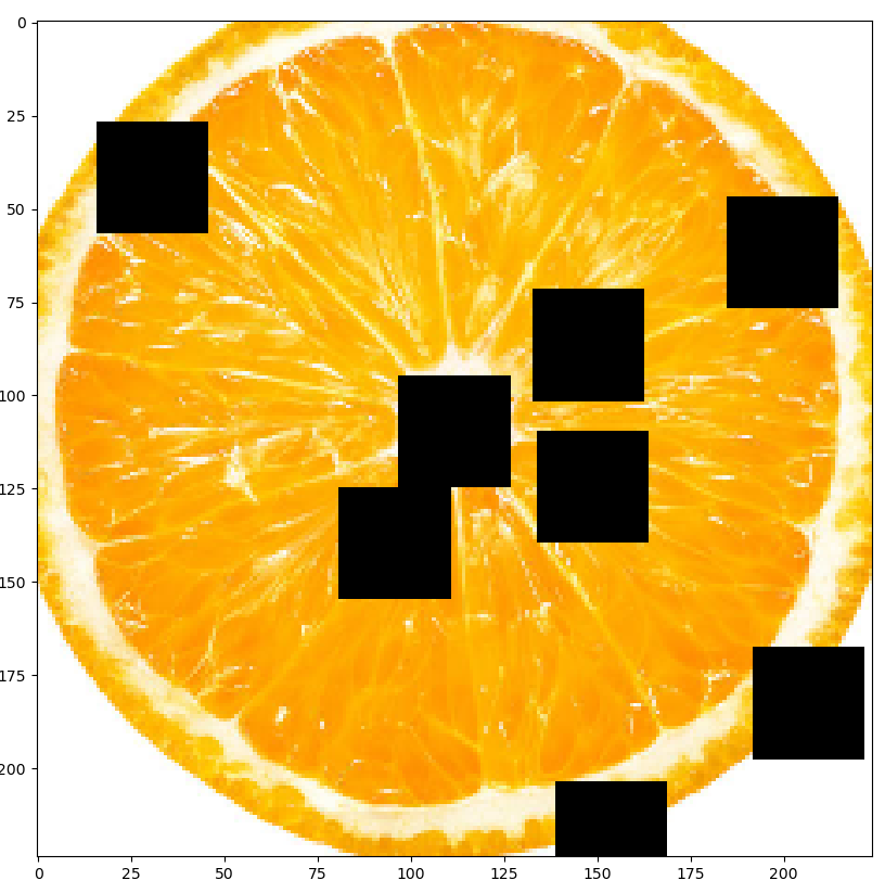
MixUp
mixup을 줘서 이미지를 겹쳐보이게 해서 개, 고양이를 0.5로 줘서 동시에 50% 확률로 보게끔하는 것이다.
두개가 더해져서 0.5의 람다값으로 겹쳐보이게 만들었다.
이것을 0.2 / 0.8로도 줄 수 있다. 그러면 하나의 상이 좀 더 뚜렷하게 보이는데 딥러닝이 봤을때는 개, 고양이가 같이 있는 사진이라고 학습할 수도 있다.
epoch가 100이상으로 되었을 때 loss값이 쭉 일자로 나오는 구간을 fitting 구간이라한다.
딥러닝에서 많이 헷갈려하는 구간에서 헷갈려하는 판단을 좀 더 잡을 수 있는 방법으로 mixup을 사용한다.
object detection, classification에서 많이 사용된다.
import torchvision
import requests
from PIL import Image
import io
import numpy as np
import cv2
import matplotlib.pyplot as plt

def get_image_from_url(url):
    response = requests.get(url)
    img_pil = Image.open(io.BytesIO(response.content)) # 이미지를 받을 때 byte로 받는 것
                                                       # byte로 받은 것을 np로 처리해야한다.
    return np.array(img_pil)

# image url
cat_url = "http://s10.favim.com/orig/160416/cute-cat-sleep-omg-Favim.com-4216420.jpeg"
dog_url = "http://s7.favim.com/orig/150714/chien-cute-dog-golden-retriever-Favim.com-2956014.jpg"

cat_img = get_image_from_url(cat_url)
dog_img = get_image_from_url(dog_url)

def mixup(x1, x2, y1, y2, lambda_=0.5):
    x = lambda_ * x1 + (1-lambda_) * x2 # 믹스업 할 때 공식, 논문에 그대로 나온다.
    y = lambda_ * y1 + (1-lambda_) * y2
    return x, y

x, y = mixup(cat_img, dog_img, np.array([1,0]), np.array([0,1]))

plt.axis('off')
plt.imshow(x.astype(int)), y
plt.show()
# np.array에서 첫번째 = cat label, 두번째(0) = dog label

# cv2.COLOR_BGR2RGB를 하지 않으면 색상이 이상하게 나온다.
# cat_img = cv2.cvtColor(cat_img, cv2.COLOR_BGR2RGB)
# cv2.imshow("Test", cat_img)
# cv2.waitKey(0)
CutMix
19년도에 나온 augmentation 기법 중 하나이다.
mixup, cutout을 합친게 cutmix이다.
똑같은 크기의 origin 이미지를 네등분으로 잘라서 붙이는 것이다.
cutmix 성능을 보면 기존의 cutout보다 많이 상승한 것을 보여준다.
mixup에서 성능이 마이너스로 떨어진 걸 볼 수 있다. 오히려 feature의 특징점을 잃어서 그렇다.
import os

import cv2.cv2
import numpy as np
import random
import cv2
import matplotlib.pyplot as plt

image_path = "./cutmix_image"
index_len = len(os.listdir(image_path))
image_list = os.listdir(image_path)

def load_image(path, index):
    image = cv2.imread(os.path.join(path, image_list[index]), cv2.cv2.IMREAD_COLOR)
    image = cv2.cvtColor(image, cv2.COLOR_BGR2RGB).astype(np.float32)
    image /= 255.0

    return image

image = load_image(image_path, 3) # 이미지 개수가 늘어나면 3을 변경해준다. 이미지는 0~3 4개이다.
image_size = image.shape[0]

def cutmix(path, index, imsize):
    w, h = imsize, imsize
    s = imsize // 2

    # 중앙값 랜덤 하게 잡기
    xc, yc = [int(random.uniform(imsize*0.25, imsize*0.75))
              for _ in range(2)] # 256 ~ 768

    indexes = [index] + [random.randint(0, index) for _ in range(3)]

    # 검은색 배경의 임의 이미지 생성 (여기다가 이미지를 붙여넣는 방식)
    return_image = np.full((imsize, imsize, 3), 1, dtype=np.float32) # 3채널짜리 이미지

    for i, index in enumerate(indexes):
        image = load_image(path, index)

        # top left
        if i == 0:
            x1a ,y1a, x2a, y2a = max(xc - w, 0), max(yc - h, 0), xc, yc
            #samll image
            x1b, y1b, x2b, y2b = w - (x2a - x1a), h - (y2a - y1a), w, h

        #top right:
        elif i == 1:
            x1a ,y1a, x2a, y2a = xc, max(yc-h, 0), min(xc+w, s*2), yc
            x1b, y1b, x2b, y2b = 0, h - (y2a - y1a), min(w, x2a - x1a), h

        # bottom left:
        elif i == 2:
            x1a ,y1a, x2a, y2a = max(xc - w, 0), yc, xc, min(s * 2, yc + h)
            x1b, y1b, x2b, y2b = w - (x2a - x1a), 0, max(xc, w), min(y2a - y1a, h)

        elif i == 3:
            x1a ,y1a, x2a, y2a = xc, yc, min(xc + w, s * 2), min(s * 2, yc + h)
            x1b, y1b, x2b, y2b = 0, 0, min(w, x2a - x1a), min(y2a - y1a, h)

        return_image[y1a:y2a, x1a:x2a] = image[y1b:y2b, x1b:x2b]
    return return_image

test = cutmix(image_path, 3, image_size)
plt.imshow(test)
plt.show()
2. 중요내용
Auto Augmentation
최적 기법을 강화학습으로 탐색한 기법이다.
잘되는 것만 자동화 학습한다.
장점 : augmentation 기법을 몰라도 여러가지 어그멘테이션을 돌릴 수 있다.
단점 : background 이미지에서 하면 안되는 것들이 있는데 (원인 경우 타원이 되는 것 등등) 그것을 방지하지 못한다.
따로 걸러야할 제약사항이 없으면 auto를 돌려도 좋다.
from PIL import Image
import cv2
import numpy as np
import torch
from torch.utils.data import Dataset
from torchvision import transforms
from matplotlib import pyplot as plt

class mycustom(Dataset):

    def __init__(self, file_path, labels, transform=None):
        self.file_path = file_path
        self.labels = labels
        self.transform = transform


    def __getitem__(self, index):
        label = self.labels[index]
        file_path = self.file_path[index]

        image = Image.open(file_path)

        if self.transform:
            image = self.transform(image)

        return image, label

torchvision_transform = transforms.Compose([
    transforms.Resize((256, 256)),
    transforms.RandomCrop(224),
    transforms.AutoAugment(),
    transforms.ToTensor()
])

train_data_set = mycustom(
    file_path=["./image/orange.jpg"],
    labels=[1],
    transform=torchvision_transform
)

for i in range(100):
    sample, _ = train_data_set[0]

plt.figure(figsize=(10, 10))
plt.imshow(transforms.ToPILImage()(sample))
plt.show()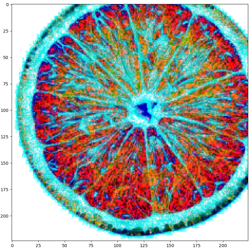
3. 학습소감
학습에서 과적합을 막기위해 사용하는 것이 Data Augmentation이라고 한다.
앞에서 배운 CutOut, MixUp, CutMix에 비해 AutoAugment나 RandAugment가 좀 더 결과적으로 좋은 것 같다는 생각이 들었다. 그 중에서도 FastAA 같은 경우에는 논문 요약을 하려고 찾아보니 카카오에서 만들었다는 것을 알게 되었다. 최신 논문에 대해서 요약하고 정리하는 습관을 잘 들여놔서 앞으로도 계속해서 잘 정리해봐야 겠다는 생각이 들었다.