
https://www.kaggle.com/c/titanic
kaggle의 타이타닉 생존 예측을 한번 해보았습니다.
데이터 가져오기
트레이닝 파일과 테스트 파일인 CSV파일 불러오기
test_df <- read.csv("test.csv")
train_df <- read.csv("train.csv")
데이터 전처리
데이터 구조 파악
| Variable | Definition | Key |
|---|---|---|
| survived | 생존여부 | 0 = No, 1 = Yes |
| pclass | 티켓 등급 | 1 = 1st, 2 = 2nd, 3 = 3rd |
| sex | 성별 | |
| Age | Age in years | |
| sibsp | # of siblings / spouses aboard the Titanic, (가족의 숫자) | |
| parch | # of parents / children aboard the Titanic (부모와 아이들) | |
| ticket | Ticket number | |
| fare | Passenger fare (여객 운임) | |
| cabin | Cabin number (객실 번호) | |
| embarked | 승선항 | C = Cherbourg, Q = Queenstown, S = Southampton |
> str(test_df)
'data.frame':	418 obs. of  11 variables:
 $ PassengerId: int  892 893 894 895 896 897 898 899 900 901 ...
 $ Pclass     : int  3 3 2 3 3 3 3 2 3 3 ...
 $ Name       : chr  "Kelly, Mr. James" "Wilkes, Mrs. James (Ellen Needs)" "Myles, Mr. Thomas Francis" "Wirz, Mr. Albert" ...
 $ Sex        : chr  "male" "female" "male" "male" ...
 $ Age        : num  34.5 47 62 27 22 14 30 26 18 21 ...
 $ SibSp      : int  0 1 0 0 1 0 0 1 0 2 ...
 $ Parch      : int  0 0 0 0 1 0 0 1 0 0 ...
 $ Ticket     : chr  "330911" "363272" "240276" "315154" ...
 $ Fare       : num  7.83 7 9.69 8.66 12.29 ...
 $ Cabin      : chr  "" "" "" "" ...
 $ Embarked   : chr  "Q" "S" "Q" "S" ...


> str(train_df)
'data.frame':	891 obs. of  12 variables:
 $ PassengerId: int  1 2 3 4 5 6 7 8 9 10 ...
 $ Survived   : int  0 1 1 1 0 0 0 0 1 1 ...
 $ Pclass     : int  3 1 3 1 3 3 1 3 3 2 ...
 $ Name       : chr  "Braund, Mr. Owen Harris" "Cumings, Mrs. John Bradley (Florence Briggs Thayer)" "Heikkinen, Miss. Laina" "Futrelle, Mrs. Jacques Heath (Lily May Peel)" ...
 $ Sex        : chr  "male" "female" "female" "female" ...
 $ Age        : num  22 38 26 35 35 NA 54 2 27 14 ...
 $ SibSp      : int  1 1 0 1 0 0 0 3 0 1 ...
 $ Parch      : int  0 0 0 0 0 0 0 1 2 0 ...
 $ Ticket     : chr  "A/5 21171" "PC 17599" "STON/O2. 3101282" "113803" ...
 $ Fare       : num  7.25 71.28 7.92 53.1 8.05 ...
 $ Cabin      : chr  "" "C85" "" "C123" ...
 $ Embarked   : chr  "S" "C" "S" "S" ...
형 변환
형을 변환해줘야 하는 것들이 있기 때문에 형변환 작업을 해줘야 한다.
train_df에서는 Survived, Pclass, Sex, Embarked를 factor형으로 해준다.
Survived factor형은 생존 여부를 "No"와 "Yes"로 바꿔준다.
train_df$Sex <- as.factor(train_df$Sex)
train_df$Embarked <- as.factor(train_df$Embarked)
train_df$Pclass <- as.factor(train_df$Pclass)
train_df$Survived <- as.factor(ifelse(train_df$Survived == 0, train_df$Survived <- "No", train_df$Survived <- "Yes"))
str(train_df)
> str(train_df)
'data.frame': 891 obs. of 12 variables:
$ PassengerId: int 1 2 3 4 5 6 7 8 9 10 ...
$ Survived : Factor w/ 2 levels "No","Yes": 1 2 2 2 1 1 1 1 2 2 ...
$ Pclass : Factor w/ 3 levels "1","2","3": 3 1 3 1 3 3 1 3 3 2 ...
$ Name : chr "Braund, Mr. Owen Harris" "Cumings, Mrs. John Bradley (Florence Briggs Thayer)" "Heikkinen, Miss. Laina" "Futrelle, Mrs. Jacques Heath (Lily May Peel)" ...
$ Sex : Factor w/ 2 levels "female","male": 2 1 1 1 2 2 2 2 1 1 ...
$ Age : num 22 38 26 35 35 NA 54 2 27 14 ...
$ SibSp : int 1 1 0 1 0 0 0 3 0 1 ...
$ Parch : int 0 0 0 0 0 0 0 1 2 0 ...
$ Ticket : chr "A/5 21171" "PC 17599" "STON/O2. 3101282" "113803" ...
$ Fare : num 7.25 71.28 7.92 53.1 8.05 ...
$ Cabin : chr "" "C85" "" "C123" ...
$ Embarked : Factor w/ 4 levels "","C","Q","S": 4 2 4 4 4 3 4 4 4 2 ...test_df 에서는 Sex, Pclass, Embarked를 factor형으로 바꿔준다.
test_df$Pclass <- as.factor(test_df$Pclass)
test_df$Embarked <- as.factor((test_df$Embarked))
test_df$Sex <- as.factor((test_df$Sex))
str(test_df)
> str(test_df)
'data.frame': 418 obs. of 11 variables:
$ PassengerId: int 892 893 894 895 896 897 898 899 900 901 ...
$ Pclass : Factor w/ 3 levels "1","2","3": 3 3 2 3 3 3 3 2 3 3 ...
$ Name : chr "Kelly, Mr. James" "Wilkes, Mrs. James (Ellen Needs)" "Myles, Mr. Thomas Francis" "Wirz, Mr. Albert" ...
$ Sex : Factor w/ 2 levels "female","male": 2 1 2 2 1 2 1 2 1 2 ...
$ Age : num 34.5 47 62 27 22 14 30 26 18 21 ...
$ SibSp : int 0 1 0 0 1 0 0 1 0 2 ...
$ Parch : int 0 0 0 0 1 0 0 1 0 0 ...
$ Ticket : chr "330911" "363272" "240276" "315154" ...
$ Fare : num 7.83 7 9.69 8.66 12.29 ...
$ Cabin : chr "" "" "" "" ...
$ Embarked : Factor w/ 3 levels "C","Q","S": 2 3 2 3 3 3 2 3 1 3 ...결측값 확인
이제 결측치가 있는지 확인해보아야한다.
# 결측값이 있는지 확인
sapply(test_df, FUN = function(x) {
  sum(is.na(x))
})

sapply(train_df, FUN = function(x) {
  sum(is.na(x))
})
> sapply(test_df, FUN = function(x) {sum(is.na(x))})
PassengerId Pclass Name Sex Age SibSp Parch Ticket Fare Cabin Embarked
0 0 0 0 86 0 0 0 1 0 0
> sapply(train_df, FUN = function(x) {sum(is.na(x))})
PassengerId Survived Pclass Name Sex Age SibSp Parch Ticket Fare Cabin Embarked
0 0 0 0 0 177 0 0 0 0 0 0
>Age에 결측치가 다량있는것을 확인했으니, 이제 결측치를 제거해야합니다.
결측치 대체
Age의 결측값을 제거할 수도 있지만, 평균값으로 대치하는 것이 더 좋은 방법이라고 생각해서 평균대치법을 사용하도록 하겠습니다.
# 결측값은 평균대치법을 활용
test_df$Age <- ifelse(is.na(test_df$Age) == TRUE, mean(test_df$Age, na.rm = TRUE), test_df$Age)
train_df$Age <- ifelse(is.na(train_df$Age) == TRUE, mean(train_df$Age, na.rm = TRUE), train_df$Age)
PassengerId Pclass Name Sex Age SibSp Parch Ticket Fare Cabin Embarked
0 0 0 0 0 0 0 0 1 0 0
PassengerId Survived Pclass Name Sex Age SibSp Parch Ticket Fare Cabin Embarked
0 0 0 0 0 0 0 0 0 0 0 0 결측치가 없어진 것을 확인할 수 있다.
성별에 따른 생존 여부
library(ggplot2)
library(scales)

ggplot_sex <- ggplot(train_df, aes(x = Survived,fill = Sex, width = .8)) +
geom_bar() + scale_y_continuous(breaks= pretty_breaks())
ggplot_sex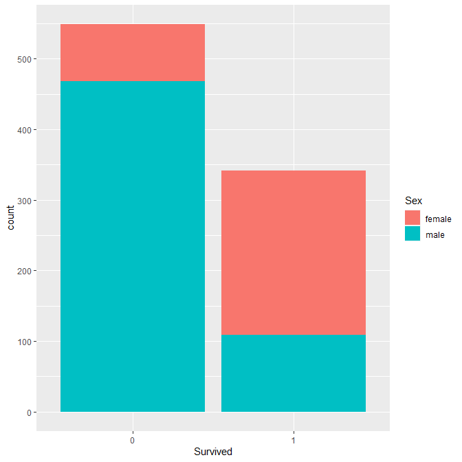
타이타닉이 침몰했을 당시에는 여성과 노약자, 아이들을 우선순위로 했다고 했는데, 실제로 여성의 생존 비율이 높은 것을 보면 어느정도 일리가 있는 자료라는 것을 증명한다.
랜덤포레스트
랜덤포레스트를 사용해서 예측 데이터를 만들어보겠습니다.
randomfor <- randomForest(Survived ~ Pclass + Age + Sex, data = train_df)
randomfor_info <- randomForest(Survived ~ Sex + Age + Pclass, data = train_df, importance = T)
importance(randomfor_info)
randomfor_pre <- predict(randomfor, newdata = test_df, type="response")
Titanic_randomFor <- data.frame(PassengerId = test_df$PassengerId, Survived = randomfor_pre)
head(Titanic_randomFor)
> head(Titanic_randomFor)
PassengerId Survived
1 892 0
2 893 0
3 894 0
4 895 0
5 896 1
6 897 0비교하기
Kaggle에서 제공하는 성별에 따른 생존여부 데이터와 예측 데이터가 얼마나 일치하는지 혼동행렬을 통해서 검사해보았습니다.
여기서 아까 우리가 test_df의 Survived를 "Yes", "No"로 설정해주었는데, 다시 0과 1로 돌려주어야합니다.
특별히 고치는 코드는 필요없고 위에서 만든 test_df 를 다시 만들어 와서 as.factor()만 해주면됩니다.
refer_df <- read.csv("gender_submission.csv")
refer_df$Survived <- as.factor(refer_df$Survived)
caret::confusionMatrix(data = Titanic_randomFor$Survived, reference = refer_df[,2])
> caret::confusionMatrix(data = Titanic_randomFor$Survived, reference = refer_df[,2])
Confusion Matrix and Statistics
Reference
Prediction 0 1
0 264 8
1 2 144
Accuracy : 0.9761
95% CI : (0.9564, 0.9885)
No Information Rate : 0.6364
P-Value [Acc > NIR] : < 2e-16
Kappa : 0.9479
Mcnemar's Test P-Value : 0.1138
Sensitivity : 0.9925
Specificity : 0.9474
Pos Pred Value : 0.9706
Neg Pred Value : 0.9863
Prevalence : 0.6364
Detection Rate : 0.6316
Detection Prevalence : 0.6507
Balanced Accuracy : 0.9699
'Positive' Class : 0 정확도인 Accuracy가 97.61% 의 결과를 얻었습니다.
다음은 로지스틱 회귀 분석을 해보겠습니다.
로지스틱 회귀
이번에는 로지스틱 회귀 분석을 활용해보겠습니다.
처음부터 해서 변수를 수정해서 해보겠습니다.
train_df <- read.csv("train.csv")
test_df <- read.csv("test.csv")
full_df <- dplyr::bind_rows(train_df, test_df)

sapply(test_df, FUN = function(x) {
    sum(is.na(x))
})

# Age 결측값은 평균 값으로 대체
train_df$Age <- ifelse(is.na(train_df$Age) == TRUE, mean(train_df$Age, na.rm = TRUE), train_df$Age)
test_df$Age <- ifelse(is.na(test_df$Age) == TRUE, mean(test_df$Age, na.rm = TRUE), test_df$Age)

#Survived 결측치는 없는 것이 당연함.
# test_df에는 Survived 변수가 없다.

nonvars = c("PassengerId", "Name", "Ticket", "Cabin", "Embarked")
train_df <- train_df[, !(names(train_df) %in% nonvars)]

glm1 <- glm(Survived ~ ., data = train_df, family = binomial)
summary(glm1)

# Fare와 Parch의 p-value가  0.05를 넘어서므로 제거를 하는게 나음.
glm2 <- glm(Survived ~ . - Parch - Fare, data = train_df, family = binomial)
summary(glm2)

logistic_pred <- predict(glm2, type = "response")
table(train_df$Survived, logistic_pred >= 0.5)
predictTest = predict(glm2, type = "response", newdata = test_df)
test_df$Survived = as.numeric(predictTest >= 0.5)
table(test_df$Survived)

predictions = data.frame(test_df[c("PassengerId", "Survived")])

refer_df <- read.csv("gender_submission.csv")
refer_df$Survived <- as.factor(refer_df$Survived)
levels(refer_df$Survived)
predictions$Survived <- as.factor(predictions$Survived)
비교하기
로지스틱 회귀 분석의 결과를 혼동 행렬을 사용해 정확도를 확인해보겠습니다.
caret::confusionMatrix(predictions$Survived, refer_df$Survived ) caret::confusionMatrix(predictions$Survived, refer_df$Survived )
Confusion Matrix and Statistics
Reference
Prediction 0 1
0 249 7
1 17 145
Accuracy : 0.9426
95% CI : (0.9158, 0.9629)
No Information Rate : 0.6364
P-Value [Acc > NIR] : < 2e-16
Kappa : 0.8777
Mcnemar's Test P-Value : 0.06619
Sensitivity : 0.9361
Specificity : 0.9539
Pos Pred Value : 0.9727
Neg Pred Value : 0.8951
Prevalence : 0.6364
Detection Rate : 0.5957
Detection Prevalence : 0.6124
Balanced Accuracy : 0.9450
'Positive' Class : 0
정확도인 Accuracy가 94.26% 의 결과를 얻었습니다.
이제 결과를 제출해 보겠습니다.
# 랜덤포레스트
write.csv(Titanic_randomFor, file="Titanic_randomFor.csv", row.names = FALSE)

# 로지스틱 회귀
write.csv(file = "logistic_pred.csv", predictions, row.names = FALSE)
결과

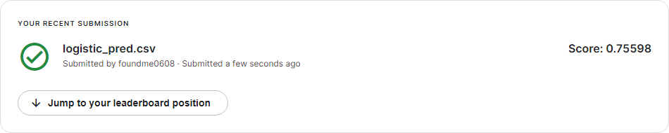
랜덤포레스트 정확도는 76% 정도가 나왔고, 로지스틱 회귀 분석은 75%정도가 나왔습니다. 미세하긴 하지만 랜덤포레스트가 아주 약간 우세합니다.
처음에 생존여부를 "Yes"와 "No"로 나눴을 때, 0점이 나와서 당황했는데,
0과 1로 다시 바꿔주니까 제대로된 결과를 얻을 수 있었습니다.