[R] 위스콘신 주 유방암 예측 및 성능평가

: ) YOUNG·2022년 5월 6일

R

목록 보기

3/8

R 데이터 분석

사용된 패키지 및 library

# library

library(mlbench)
library(C50)
library(gmodels)
library(caret)
library(Epi)
library(tidyverse)

> library(tidyverse)
-- Attaching packages ------------------------------------------------------------------------------------------------------------------------------------------------------------------------------- tidyverse 1.3.1 --v tibble  3.1.6     v dplyr   1.0.8
v tidyr   1.2.0     v stringr 1.4.0
v readr   2.1.2     v forcats 0.5.1
v purrr   0.3.4
-- Conflicts ---------------------------------------------------------------------------------------------------------------------------------------------------------------------------------- tidyverse_conflicts() --x dplyr::filter() masks stats::filter()
x dplyr::lag()    masks stats::lag()
x purrr::lift()   masks caret::lift()
Warning messages:
1: package 'tidyverse' was built under R version 4.1.3
2: package 'tibble' was built under R version 4.1.3
3: package 'tidyr' was built under R version 4.1.3
4: package 'readr' was built under R version 4.1.3
5: package 'purrr' was built under R version 4.1.3
6: package 'dplyr' was built under R version 4.1.3
7: package 'stringr' was built under R version 4.1.3
8: package 'forcats' was built under R version 4.1.3

데이터 설명

Format

Col	Name	describ
[,1]	Id	Sample code number (환자 고유 번호)
[,2]	Cl.thickness	Clump Thickness (뭉침 두께 정도)
[,3]	Cell.size	Uniformity of Cell Size (세포 크기의 균일도)
[,4]	Cell.shape	Uniformity of Cell Shape (세포 모양의 균일도)
[,5]	Marg.adhesion	Marginal Adhesion (밀착도)
[,6]	Epith.c.size	Single Epithelial Cell Size (단일 상피 세포 크기)
[,7]	Bare.nuclei	Bare Nuclei (세포 핵)
[,8]	Bl.cromatin	Bland Chromatin (염색질 건조도)
[,9]	Normal.nucleoli	Normal Nucleoli (핵소체 정상도)
[,10]	Mitoses	Mitoses (분열도)
[,11]	Class	Class (양성 음성 여부)

데이터 호출 및 기초 통계 확인

data(BreastCancer)
df <- BreastCancer

head(df, 10)
summary(df)
str(df)

# 앞쪽 10줄 확인
> head(df, 10)
        Id Cl.thickness Cell.size Cell.shape Marg.adhesion Epith.c.size
1  1000025            5         1          1             1            2
2  1002945            5         4          4             5            7
3  1015425            3         1          1             1            2
4  1016277            6         8          8             1            3
5  1017023            4         1          1             3            2
6  1017122            8        10         10             8            7
7  1018099            1         1          1             1            2
8  1018561            2         1          2             1            2
9  1033078            2         1          1             1            2
10 1033078            4         2          1             1            2
   Bare.nuclei Bl.cromatin Normal.nucleoli Mitoses     Class
1            1           3               1       1    benign
2           10           3               2       1    benign
3            2           3               1       1    benign
4            4           3               7       1    benign
5            1           3               1       1    benign
6           10           9               7       1 malignant
7           10           3               1       1    benign
8            1           3               1       1    benign
9            1           1               1       5    benign
10           1           2               1       1    benign



# 기초 통계 확인
> summary(df)
      Id             Cl.thickness   Cell.size     Cell.shape  Marg.adhesion
 Length:699         1      :145   1      :384   1      :353   1      :407  
 Class :character   5      :130   10     : 67   2      : 59   2      : 58  
 Mode  :character   3      :108   3      : 52   10     : 58   3      : 58  
                    4      : 80   2      : 45   3      : 56   10     : 55  
                    10     : 69   4      : 40   4      : 44   4      : 33  
                    2      : 50   5      : 30   5      : 34   8      : 25  
                    (Other):117   (Other): 81   (Other): 95   (Other): 63
  Epith.c.size  Bare.nuclei   Bl.cromatin  Normal.nucleoli    Mitoses
 2      :386   1      :402   2      :166   1      :443     1      :579
 3      : 72   10     :132   3      :165   10     : 61     2      : 35
 4      : 48   2      : 30   1      :152   3      : 44     3      : 33
 1      : 47   5      : 30   7      : 73   2      : 36     10     : 14
 6      : 41   3      : 28   4      : 40   8      : 24     4      : 12  
 5      : 39   (Other): 61   5      : 34   6      : 22     7      :  9
 (Other): 66   NA's   : 16   (Other): 69   (Other): 69     (Other): 17
       Class
 benign   :458
 malignant:241
 
 
 # 데이터 형 확인
 > str(df)
'data.frame':   699 obs. of  11 variables:
 $ Id             : chr  "1000025" "1002945" "1015425" "1016277" ...
 $ Cl.thickness   : Ord.factor w/ 10 levels "1"<"2"<"3"<"4"<..: 5 5 3 6 4 8 1 2 2 4 ...
 $ Cell.size      : Ord.factor w/ 10 levels "1"<"2"<"3"<"4"<..: 1 4 1 8 1 10 1 1 1 2 ...
 $ Cell.shape     : Ord.factor w/ 10 levels "1"<"2"<"3"<"4"<..: 1 4 1 8 1 10 1 2 1 1 ...
 $ Marg.adhesion  : Ord.factor w/ 10 levels "1"<"2"<"3"<"4"<..: 1 5 1 1 3 8 1 1 1 1 ...
 $ Epith.c.size   : Ord.factor w/ 10 levels "1"<"2"<"3"<"4"<..: 2 7 2 3 2 7 2 2 2 2 ...
 $ Bare.nuclei    : Factor w/ 10 levels "1","2","3","4",..: 1 10 2 4 1 10 10 1 1 1 ...
 $ Bl.cromatin    : Factor w/ 10 levels "1","2","3","4",..: 3 3 3 3 3 9 3 3 1 2 ...
 $ Normal.nucleoli: Factor w/ 10 levels "1","2","3","4",..: 1 2 1 7 1 7 1 1 1 1 ...
 $ Mitoses        : Factor w/ 9 levels "1","2","3","4",..: 1 1 1 1 1 1 1 1 5 1 ...
 $ Class          : Factor w/ 2 levels "benign","malignant": 1 1 1 1 1 2 1 1 1 1 ...

Id(환자 고유 번호) 제거

Id변수는 예측하는데 필요하지 않기 때문에 제거하겠습니다.

df <- df[-1]

Class를 제외한 9개의 변수들 (
Cl.thickness,
Cell.size,
Cell.shape,
Marg.adhesion,
Epth.c.size,
Bare.nuclei,
Bl.cromatin,
Normal.nucleoli,
Mitoses ) 이 현재 factor형으로 되어있어서 수치형인 numeric으로 바꿔주겠습니다.


# 9개의 변수 factor형을 numeric형으로 바꿈
df <- cbind(lapply(df[-10], function(x) as.numeric(as.character(x))), df[10])

str(df)

출력

# facotr형에서 num 형으로 전환된 것을 확인
> str(df)
'data.frame':   699 obs. of  10 variables:
 $ Cl.thickness   : num  5 5 3 6 4 8 1 2 2 4 ...
 $ Cell.size      : num  1 4 1 8 1 10 1 1 1 2 ...
 $ Cell.shape     : num  1 4 1 8 1 10 1 2 1 1 ...
 $ Marg.adhesion  : num  1 5 1 1 3 8 1 1 1 1 ...
 $ Epith.c.size   : num  2 7 2 3 2 7 2 2 2 2 ...
 $ Bare.nuclei    : num  1 10 2 4 1 10 10 1 1 1 ...
 $ Bl.cromatin    : num  3 3 3 3 3 9 3 3 1 2 ...
 $ Normal.nucleoli: num  1 2 1 7 1 7 1 1 1 1 ...
 $ Mitoses        : num  1 1 1 1 1 1 1 1 5 1 ...
 $ Class          : Factor w/ 2 levels "benign","malignant": 1 1 1 1 1 2 1 1 1 1 ...

train data와 test data 생성

train data와 test data를 만들기 위해서 기존 하나의 데이터를 분리합니다.

단순랜덤 추출방식으로 비율은 train 7 : test 3 으로 분리합니다.


# train데이터와 test데이터 2개의 집단으로 분리
# 랜덤으로 훈련 7: 테스트 3의 비율로 분리
set.seed(202205)
samples <- sample(nrow(df), 0.7 * nrow(df))
train <- df[samples, ]
test <- df[-samples, ]

dim(train)
dim(test)

table(train$Class)
table(test$Class)

출력

> dim(train)
[1] 489  10 

> dim(test)
[1] 210  10

> table(train$Class)

   benign malignant 
      319       170
      
> table(test$Class)

   benign malignant
      139        71

train 과 test가 잘 분리되었습니다.

Class 변수에서 benign은 양성을 의미하고 malignant는 음성을 의미합니다.

의사결정나무

dctree <- C5.0(formula = Class ~ . , data = df.train)

> dctree

Call:
C5.0.formula(formula = Class ~ ., data = train)

Classification Tree
Number of samples: 489
Number of predictors: 9

Tree size: 8

Non-standard options: attempt to group attributes

Class의 양성 음성의 범주로
Class가 종속변수인 formula를 만들고 나머지는 독립변수로 생성해서 의사결정나무를 만들었습니다.

dctree.pred <- predict(dctree, newdata = test, type = "class")

이제 의사결정나무 모델로 예측한 값이 생성되었습니다.

이번에는 검증하기 전에 마지막으로 해당 의사결정나무를 통해 예측한 데이터를 CrossTable로 생성해보겠습니다.

이 테이블로 pred모델의 실제 Class의 값과 예측한 Class의 값을 살펴 볼 수 있습니다.


> CrossTable(test$Class, dctree.pred, prob.chisq = FALSE, dnn = c("Actual", "P$


   Cell Contents
|-------------------------|
|                       N |
| Chi-square contribution |
|           N / Row Total |
|           N / Col Total |
|         N / Table Total |
|-------------------------|


Total Observations in Table:  210


|             | Predicted
|      Actual |    benign | malignant | Row Total |
|-------------|-----------|-----------|-----------|
|      benign |       128 |        11 |       139 | 
|             |    18.893 |    31.972 |           |
|             |     0.921 |     0.079 |     0.662 |
|             |     0.970 |     0.141 |           |
|             |     0.610 |     0.052 |           |
|-------------|-----------|-----------|-----------|
|   malignant |         4 |        67 |        71 |
|             |    36.987 |    62.594 |           |
|             |     0.056 |     0.944 |     0.338 |
|             |     0.030 |     0.859 |           | 
|             |     0.019 |     0.319 |           |
|-------------|-----------|-----------|-----------|
|Column Total |       132 |        78 |       210 |
|             |     0.629 |     0.371 |           |
|-------------|-----------|-----------|-----------|

이제 마지막으로 실제 데이터와 예측한데이터가 어느정도의 정확도를 가지고 있는지 혼동행렬과 ROC curve를 통해서 검증해보겠습니다.

Confusion Matrix (혼동행렬)


# caret의 혼동행렬을 통한 정확도 계산
# 음성 = positive
caret::confusionMatrix(dctree.pred, test$Class, positive = "malignant")

혼동 행렬 출력


> caret::confusionMatrix(dctree.pred, test$Class, positive = "malignant")
Confusion Matrix and Statistics

           Reference
Prediction  benign malignant
  benign       128         4
  malignant     11        67

               Accuracy : 0.9286
                 95% CI : (0.8849, 0.9595)
    No Information Rate : 0.6619
    P-Value [Acc > NIR] : <2e-16

                  Kappa : 0.8442

 Mcnemar's Test P-Value : 0.1213

            Sensitivity : 0.9437
            Specificity : 0.9209
         Pos Pred Value : 0.8590
         Neg Pred Value : 0.9697
             Prevalence : 0.3381
         Detection Rate : 0.3190
   Detection Prevalence : 0.3714
      Balanced Accuracy : 0.9323

       'Positive' Class : malignant

혼동행렬 지표에서 해당 부분은 긍정이 양성인데, 아래에 있어서 계산을 잘못할 경우 오답을 얻을 수 있기 때문에 어떤게 긍정을 나타내는지 잘 확인해야 합니다.

여기서는 Positive(긍정)이 아래에 있기 때문에 FP와 TP가 아래쪽으로 향해 있습니다.

	Reference(실제)	=========
Predict(예측)	TN	FN
=========	FP	TP

👇 수치화

	Reference(실제)	=========
Predict(예측)	128	4
=========	11	67

계산을 해보면
Accuracy(정확도) = (TP + FP) / (TP + FP + TN + FN) = (67 + 11) / 210 = 0.9285714286

결과 값 0.9286과 일치합니다.

ROC 곡선

마지막으로 ROC곡선을 살펴보겠습니다.


bc.C50.pred <- predict(dctree, newdata = test, type="prob")
result <- ROC(test = bc.C50.pred[, 2], stat = test$Class, MI=FALSE, main = "ROC Curve")
result

그래프가 정상적으로 출력되었습니다.

AUROC, 그래프 곡선 아래의 면적을 통해서 성능을 평가할 수 있습니다.

result 결과 출력에서 AUC의 값을 확인하면 됩니다.


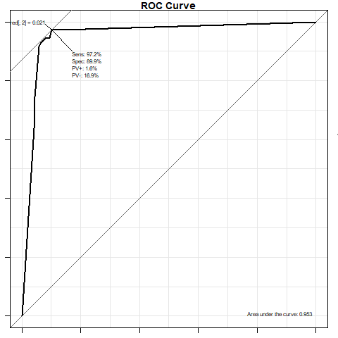
> result
$res
                         sens      spec        pvp       pvn bc.C50.pred[, 2]
                    1.0000000 0.0000000        NaN 0.6619048             -Inf
0.00121134336421238 0.9718310 0.8633094 0.01639344 0.2159091      0.001211343
0.0207146806875534  0.9718310 0.8992806 0.01574803 0.1686747      0.020714681
0.03476482629776    0.9436620 0.9064748 0.03076923 0.1625000      0.034764826
0.0756140413811419  0.9436620 0.9136691 0.03053435 0.1518987      0.075614041
0.110521769157897   0.9436620 0.9208633 0.03030303 0.1410256      0.110521769
0.634764827153434   0.9295775 0.9352518 0.03703704 0.1200000      0.634764827
0.782549420992533   0.9154930 0.9424460 0.04379562 0.1095890      0.782549421
0.928336108741788   0.7464789 0.9568345 0.11920530 0.1016949      0.928336109
0.949819097152123   0.6760563 0.9568345 0.14743590 0.1111111      0.949819097
0.961018262815205   0.0000000 1.0000000 0.33809524       NaN      0.961018263

$AUC
[1] 0.9532374

$lr

Call:  glm(formula = stat ~ test, family = binomial)

Coefficients:
(Intercept)         test
     -3.584        5.853

Degrees of Freedom: 209 Total (i.e. Null);  208 Residual
Null Deviance:      268.7
Residual Deviance: 93.28        AIC: 97.28

AUC는 1에 가까울수록 좋은 모형으로 평가합니다.
AUC의 결과값이 0.95의 값으로, 좋은 모형이라고 할 수 있습니다.