5장. 차원 축소를 사용한 데이터 압축 - 2

커널 PCA를 사용하여 비선형 매핑
💡 많은 머신 러닝 알고리즘은 입력 데이터가 선형적으로 구분 가능하다는 가정을 한다
💡 선형적으로 완벽하게 분리되지 못한 이유를 잡음 때문이라고 가정한다
- 비선형 문제를 해결하기 위해 클래스가 선형으로 구분되는 새로운 고차원 특성 공간으로 투영할 수 있다
- 커널 PCA를 통한 비선형 매핑을 수행하여 데이터를 고차원 공간으로 변환
- 하지만 이 방법들은 계산 비용이 매우 비싸다
-
커널 트릭( Kernel trick )이 등장하게 된다
-
커널 트릭을 사용하면 원본 특성 공간에서 두 고차원 특성 벡터의 유사도를 계산할 수 있다
-
기본적으로 커널 함수는 두 벡터 사이의 점곱을 계산할 수 있는 함수
-
가장 널리 사용되는 커널
- 다항 커널
- 하이퍼볼릭 탄젠트( hyperbolic tangent ) ( 시그모이드 ) 커널
- 방사 기저 함수( Radial Basis Function, RBF ) 또는 가우시안 커널
-
RBF 커널 PCA를 구현하기 위한 단계 정의
-
커널 ( 유사도 ) 행렬 를 다음 식으로 계산
-
다음 식을 사용하여 커널 행렬 를 중앙에 맞춘다
-
고윳값 크기대로 내림차순으로 정렬하여 정렬하여 중앙에 맞춘 커널 행렬에서 최상위 개의 고유 벡터를 고른다
- 표준 PCA와 다르게 고유 벡터는 주성분 축이 아니며, 이미 축에 투영된 샘플
-
📍 파이썬으로 커널 PCA 구현
from scipy.spatial.distance import pdist, squareform
from numpy import exp
from scipy.linalg import eigh
import numpy as np
def rbf_kernel_pca(x, gamma, n_components):
'''
RBF 커널 PCA 구현
매개변수
--------
x: { 넘파이 ndarray }, shape = [n_samples, n_features]
gamma: float
RBF 커널 튜닝 매개변수
n_components: int
반환할 주성분 개수
반환값
-------
x_pc: { 넘파이 ndarray }, shape = [n_samples, k_features]
투영된 데이터셋
'''
# MxN 차원의 데이터셋에서 샘플간의 유클리디안 거리의 제곱을 계산
sq_dists = pdist(x, 'sqeuclidean')
# 샘플 간의 거리를 정방 대칭 행렬로 변환
mat_sq_dists = squareform(sq_dists)
# 커널 행렬을 계산
k = exp(-gamma * mat_sq_dists)
# 커널 행렬을 중앙에 맞춘다
n = k.shape[0]
one_n = np.ones((n, n)) / n
k = k - one_n.dot(k) - k.dot(one_n) + one_n.dot(k).dot(one_n)
# 중앙에 맞춰진 커널 행렬의 고윳값과 고유 벡터 구하기
# scipy.linalg.eigh 함수는 오름차순으로 반환
eigvals, eigvecs = eigh(k)
eigvals, eigvecs = eigvals[::-1], eigvecs[:, ::-1]
# 최상위 k개의 고유 벡터를 선택( 투영 결과 )
x_pc = np.column_stack([eigvecs[:, i] for i in range(n_components)])
return x_pc예제 1: 반달 모양 구분하기
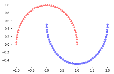
rbf_kernel_pca함수를 비선형 데이터셋에 적용- 두 개의 반달 모양을 띤 100개의 샘플로 구성된 2차원 데이터셋을 사용
📍 반달 시각화
from sklearn.datasets import make_moons

x, y = make_moons(n_samples=100, random_state=123)
plt.scatter(x[y==0, 0], x[y==0, 1],
           color='r', marker='^', alpha=0.5)
plt.scatter(x[y==1, 0], x[y==1, 1],
           color='b', marker='o', alpha=0.5)

plt.show()

~~>
📍 기본 PCA의 주성분에 데이터셋 투영
from sklearn.decomposition import PCA

scikit_pca = PCA(n_components=2)
x_spca = scikit_pca.fit_transform(x)
fig, ax = plt.subplots(nrows=1, ncols=2, figsize=(7, 3))
ax[0].scatter(x_spca[y==0, 0], x_spca[y==0, 1],
             color='r', marker='^', alpha=0.5)
ax[0].scatter(x_spca[y==1, 0], x_spca[y==1, 1],
             color='b', marker='o', alpha=0.5)

ax[1].scatter(x_spca[y==0, 0], np.zeros((50, 1))+0.02,
             color='r', marker='^', alpha=0.5)
ax[1].scatter(x_spca[y==1, 0], np.zeros((50, 1))-0.02,
             color='b', marker='o', alpha=0.5)

ax[0].set_xlabel('PC 1')
ax[0].set_ylabel('PC 2')

ax[1].set_ylim([-1, 1])
ax[1].set_yticks([])
ax[1].set_xlabel('PC 1')

plt.show()

~~>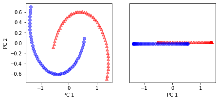
📍 커널 PCA 함수 rbf_kernel_pca
x_kpca = rbf_kernel_pca(x, gamma=15, n_components=2)
fig, ax = plt.subplots(nrows=1, ncols=2, figsize=(7,3))
ax[0].scatter(x_kpca[y==0, 0], x_kpca[y==0, 1],
             color='r', marker='^', alpha=0.5)
ax[0].scatter(x_kpca[y==1, 0], x_kpca[y==1, 1],
             color='b', marker='o', alpha=0.5)
ax[1].scatter(x_kpca[y==0, 0], np.zeros((50, 1))+0.02,
             color='r', marker='^', alpha=0.5),
ax[1].scatter(x_kpca[y==1, 0], np.zeros((50, 1))-0.02,
             color='b', marker='o', alpha=0.5)

ax[0].set_xlabel('PC 1')
ax[0].set_ylabel('PC 2')
ax[1].set_ylim([-1, 1])
ax[1].set_yticks([])
ax[1].set_xlabel('PC 1')

plt.tight_layout()
plt.show()

~~>
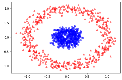
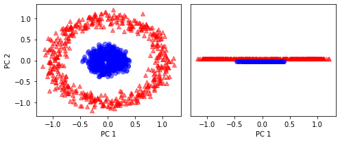
예제 2: 동심원 분리하기
from sklearn.datasets import make_circles

x, y = make_circles(n_samples=1000,
                   random_state=123, noise=0.1, factor=0.2)
plt.scatter(x[y==0, 0], x[y==0, 1],
           color='r', marker='^', alpha=0.5)
plt.scatter(x[y==1, 0], x[y==1, 1],
           color='b', marker='o', alpha=0.5)
plt.tight_layout()
plt.show()

~~>
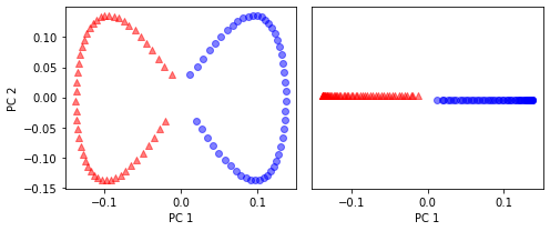
📍 기본 PCA 적용
scikit_pca = PCA(n_components=2)
x_spca = scikit_pca.fit_transform(x)
fig, ax = plt.subplots(nrows=1, ncols=2, figsize=(7,3))
ax[0].scatter(x_spca[y==0, 0], x_spca[y==0, 1],
             color='r', marker='^', alpha=0.5)
ax[0].scatter(x_spca[y==1, 0], x_spca[y==1, 1],
             color='b', marker='o', alpha=0.5)
ax[1].scatter(x_spca[y==0, 0], np.zeros((500, 1))+0.02,
             color='r', marker='^', alpha=0.5)
ax[1].scatter(x_spca[y==1, 0], np.zeros((500, 1))-0.02,
             color='b', marker='o', alpha=0.5)

ax[0].set_xlabel('PC 1')
ax[0].set_ylabel('PC 2')
ax[1].set_ylim([-1, 1])
ax[1].set_yticks([])
ax[1].set_xlabel('PC 1')

plt.tight_layout()
plt.show()

~~>
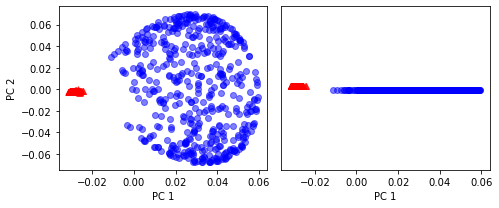
📍 RBF 커널 PCA
x_kpca = rbf_kernel_pca(x, gamma=15, n_components=2)
fig, ax = plt.subplots(nrows=1, ncols=2, figsize=(7,3))
ax[0].scatter(x_kpca[y==0, 0], x_kpca[y==0, 1],
             color='r', marker='^', alpha=0.5)
ax[0].scatter(x_kpca[y==1, 0], x_kpca[y==1, 1],
             color='b', marker='o', alpha=0.5)
ax[1].scatter(x_kpca[y==0, 0], np.zeros((500, 1))+0.02,
             color='r', marker='^', alpha=0.5)
ax[1].scatter(x_kpca[y==1, 0], np.zeros((500, 1))-0.02,
             color='b', marker='o', alpha=0.5)

ax[0].set_xlabel('PC 1')
ax[0].set_ylabel('PC 2')
ax[1].set_ylim([-1, 1])
ax[1].set_yticks([])
ax[1].set_xlabel('PC 1')

plt.tight_layout()
plt.show()

~~>
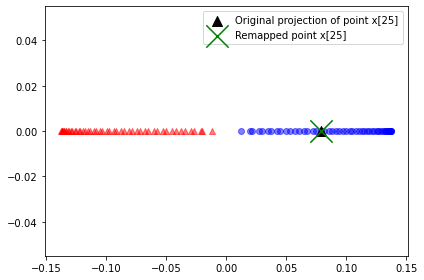
새로운 데이터 포인트 우영
- 훈련 데이터셋에 포함되지 않았던 새로운 데이터 포인트를 투영하는 방법
from scipy.spatial.distance import pdist, squareform
from numpy import exp
from scipy.linalg import eigh
import numpy as np
def rbf_kernel_pca(x, gamma, n_components):
'''
RBF 커널 PCA 구현
매개변수
----------
X: { 넘파이 ndarray }, shape = [n_samples, n_features]
gamma: float
RBF 커널 튜닝 매개변수
n_components: int
반환할 주성분 개수
반환값
--------
alpha: { 넘파이 ndarray }, shape = [n_samples, k_features]
투영된 데이터셋
lambdas: list
고윳값
'''
# MxN 차원의 데이터셋에서 샘플 간의 유클라디안 거리의 제곱을 계산
sq_dists = pdist(x, 'sqeuclidean')
# 샘플 간의 거리를 정방 대칭 행렬로 변환
mat_sq_dists = squareform(sq_dists)
# 커널 행렬을 계산
k = exp(-gamma * mat_sq_dists)
# 커널 행렬을 중앙에 맞추기
n = k.shape[0]
one_n = np.ones((n, n)) / n
k = k - one_n.dot(k) - k.dot(one_n) + one_n.dot(k).dot(one_n)
# 중앙에 맞춰진 커널 행렬의 고윳값과 고유 벡터를 구하기
# scipy.linalg.eigh 함수는 오름차순으로 반환
eigvals, eigvecs = eigh(k)
eigvals, eigvecs = eigvals[:: -1], eigvecs[:, :: -1]
# 최상위 k개의 고유 벡터를 선택( 투영 결과 )
alphas = np.column_stack([eigvecs[:, i] for i in range(n_components)])
# 고유 벡터에 상응하는 고윳값을 선택
lambdas = [eigvals[i] for i in range(n_components)]
return alphas, lambdas📍 수정된 커널 PCA 구현을 사용하여 1차우너 부분 공간에 투영
x, y = make_moons(n_samples=100, random_state=123)
alphas, lambdas = rbf_kernel_pca(x, gamma=15, n_components=1)
x_new = x[25]
x_new
~~>
array([1.8713, 0.0093])x_proj = alphas[25] # 원본 투영
x_proj
~~>
array([0.0788])def project_x(x_new, x, gamma, alphas, lambdas):
pair_dist = np.array([np.sum((x_new-row)**2) for row in x])
k = np.exp(-gamma * pair_dist)
return k.dot(alphas / lambdas)📍 project_x 함수를 사용하여 새로운 데이터 샘플 투영
x_reproj = project_x(x_new, x, gamma=15, alphas=alphas, lambdas=lambdas)
x_reproj

~~>
array([0.0788])
📍 시각화
plt.scatter(alphas[y==0, 0], np.zeros((50)),
           color='r', marker='^', alpha=0.5)
plt.scatter(alphas[y==1, 0], np.zeros((50)),
           color='b', marker='o', alpha=0.5)
plt.scatter(x_proj, 0, color='black',
           label='Original projection of point x[25]',
           marker='^', s=100)
plt.scatter(x_reproj, 0, color='g',
           label='Remapped point x[25]',
           marker='x', s=500)
plt.legend(scatterpoints=1)
plt.tight_layout()
plt.show()

~~>
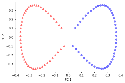
사이킷런의 커널 PCA
sklearn.decomposition모듈 아래 커널 PCA 클래스를 구현kernel매개변수로 커널의 종류를 지정
from sklearn.decomposition import KernelPCA

x, y = make_moons(n_samples=100, random_state=123)
scikit_kpca = KernelPCA(n_components=2, kernel='rbf', gamma=15)
x_skernpca = scikit_kpca.fit_transform(x)
📍 시각화
plt.scatter(x_skernpca[y==0, 0], x_skernpca[y==0, 1],
           color='r', marker='^', alpha=0.5)
plt.scatter(x_skernpca[y==1, 0], x_skernpca[y==1, 1],
           color='b', marker='o', alpha=0.5)
plt.xlabel('PC 1')
plt.ylabel('PC 2')
plt.tight_layout()

plt.show()

~~>

data science!!, data analyst!! ///// hello world