import tensorflow as tf텐서플로우를 통해 딥러닝을 하는 방법밖에 모르기에 텐서플로우를 import해준다!!
mnist = tf.keras.datasets.mnist

(x_train, y_train),(x_test,y_test) = mnist.load_data()
x_train, x_test = x_train/ 255.0, x_test / 255.0
MNIST에 내포되어 있는 데이터를 기반으로 분석하려고 한다.
딥러닝을 해주기 위해 x_train, y_train,x_test,y_test를 만들어줬다.
model = tf.keras.models.Sequential([
    tf.keras.layers.Flatten(input_shape=(28,28)),
    tf.keras.layers.Dense(1000,activation='relu'),
    tf.keras.layers.Dense(10,activation='softmax')
])

model.compile(optimizer='adam',
              loss='sparse_categorical_crossentropy',
              metrics=['accuracy'])
layers를 구분해줬고 relu,softmax를 활용하였다.
%%time

hist = model.fit(x_train,y_train,validation_data=(x_test,y_test),epochs=10,batch_size=100,verbose=1)
시간 지남에 따라 확인가능할 수 있도록 설정을 해두었고, 만든 model을 fit했다.
acc와 loss 그려보기
import matplotlib.pyplot as plt
%matplotlib inline
plot_target = ['loss','val_loss','accuracy','val_accuracy']
plt.figure(figsize=(12,8))
for each in plot_target:
plt.plot(hist.history[each],label=each)
plt.legend()
plt.grid()
plt.show()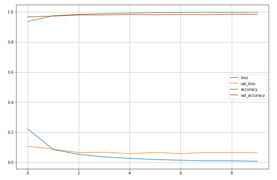
score = model.evaluate(x_test,y_test)
print('Test loss:',score[0])
print('test accuracy:',score[1])
313/313 [==============================] - 1s 3ms/step - loss: 0.0642 - accuracy: 0.9837
Test loss: 0.06417490541934967
test accuracy: 0.9836999773979187
- 위의 결과값을 보면 머신러닝에서 할 때는 93%정도 나왔던 결과대비 약 5% 향상되었다!!
import numpy as np

predicted_result = model.predict(x_test)
predicted_labels = np.argmax(predicted_result,axis=1)
predicted_labels[:10]
array([7, 2, 1, 0, 4, 1, 4, 9, 5, 9], dtype=int64)
wrong_result =[]

for n in range(0,len(y_test)):
    if predicted_labels[n] !=y_test[n]:
        wrong_result.append(n)

len(wrong_result)
wrong_result가 총 163개라고 나왔다.
시각화를 해보자~
import random

samples = random.choices(population = wrong_result,k=16)
plt.figure(figsize=(14,12))
for idx, n in enumerate(samples):
plt.subplot(4,4,idx+1)
plt.imshow(x_test[n].reshape(28,28),cmap='Greys')
plt.title('Label:' + str(y_test[n]) + ' | predict :'+ str(predicted_labels[n]))
plt.axis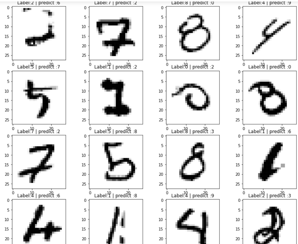
MNIST fashion
import tensorflow as tf

fashion_mnist = tf.keras.datasets.fashion_mnist

(x_train, y_train),(x_test,y_test) = fashion_mnist.load_data()
x_train, x_test = x_train/255, x_test/255
방식은 위에 방식과 동일하다,,
samples = random.choices(population=range(0,len(y_train)),k=16)

plt.figure(figsize=(14,12))

for idx, n in enumerate(samples):
    plt.subplot(4,4,idx+1)
    plt.imshow(x_train[n].reshape(28,28),cmap='Greys')
    plt.title('Label:' + str(y_train[n]))
    plt.axis('off')
plt.show()
%%time

hist = model.fit(x_train,y_train,validation_data=(x_test,y_test),epochs=10,batch_size=100,verbose=1)
plot_target = ['loss','val_loss','accuracy','val_accuracy']
plt.figure(figsize=(12,8))
for each in plot_target:
plt.plot(hist.history[each],label=each)
plt.legend()
plt.grid()
plt.show()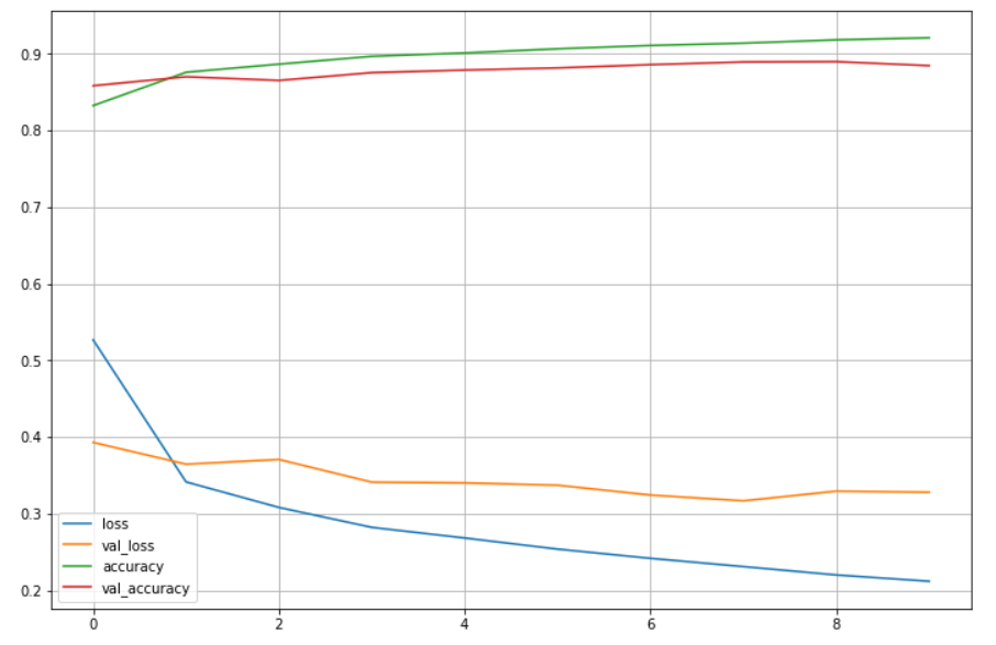
- 학습이 잘되어보이지만 val_loss와 train loss 사이에 간격이 벌어진다.

문과생 데이터사이언티스트되기 프로젝트