Basic ML_1

1. Machine Learning의 기본 개념

Supervised Learning(지도 학습) : 하나의 정해져 있는 데이터(레이블)를 갖고 교육시키는 것.
Unsupervised Learning(비지도 학습) : 일일이 레이블을 줄 수 없는 경우 유사한 데이터를 스스로 학습시키는 것.

✔ training data set?
Supervised Learning(지도학습)에서 컴퓨터가 학습할 수 있도록 정해진 데이터의 집합

• Supervised Learning의 종류
  regression : 예측 변수(feature)를 사용해 최종 결과를 예측
  binary classification : yes or no 둘 중 하나로 분류
  multi-label classification : 다양한 결과로 분류

2. Simple Linear Regression

Linear Regression : 데이터를 가장 잘 대변하는 직선의 방정식을 찾는 것.
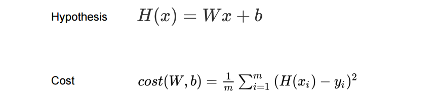
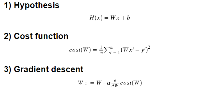
H(x) = Wx + b ⇒ Hypothesis 함수
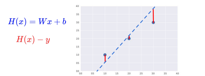H(x) - y = cost
즉 가설 데이터 - 실제 데이터 = cost(=loss, error)가 작을수록 실제 데이터를 가장 잘 대변했다.
cost가 -인 값도 있기 때문에 오차를 제곱하여 평균을 낸다.
cost function을 minimize하는 것이 목표

3. Linear Regression TensorFlow

import tensorflow as tf
import numpy as np

# Data
x_data = [1, 2, 3, 4, 5]
y_data = [1, 2, 3, 4, 5]

# W, b initialize
W = tf.Variable(2.9)  # 임의의 초기값을 지정
b = tf.Variable(0.5)

# W, b update
for i in range(100):
    # Gradient descent
    with tf.GradientTape() as tape:
        hypothesis = W * x_data + b
        cost = tf.reduce_mean(tf.square(hypothesis - y_data))
        # reduce_mean() : 평균
        # square() : 값을 제곱
    W_grad, b_grad = tape.gradient(cost, [W, b])
    # W,b에 대한 미분값을 구하여(cost) 튜플로 반환. w의 grad는 W_grad, b의 grad는 b_grad
    W.assign_sub(learning_rate * W_grad)
    b.assign_sub(learning_rate * b_grad)
    # W_grad, b_grad의 기울기를 learning_rate에 따라 얼마만큼 반영할지 결정
    if i % 10 == 0:
      print("{:5}|{:10.4f}|{:10.4f}|{:10.6f}".format(i, W.numpy(), b.numpy(), cost))

print()

# predict
print(W * 5 + b)
print(W * 2.5 + b)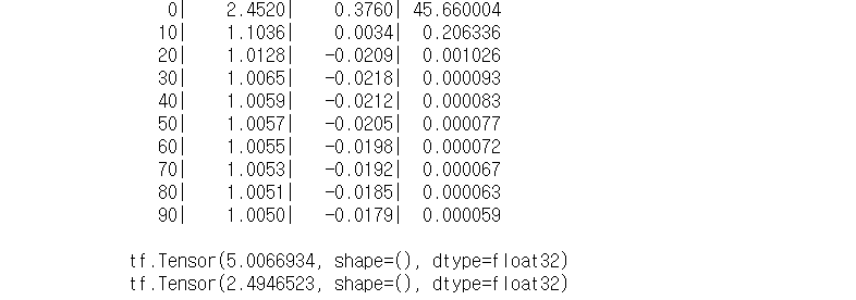

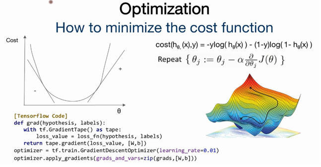
4. Minimize cost(Gradient Descent)

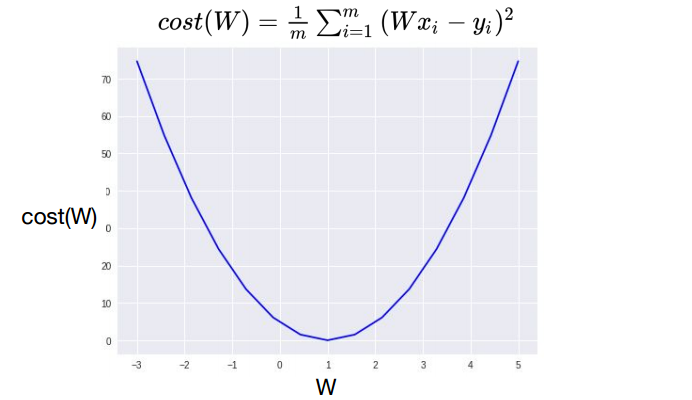cost가 가장 작게 되는 W값 구하기.
최저점을 찾는 알고리즘으로 경사를 따라 내려오면서 최소점을 찾는 알고리즘
⇒ gradient descent algorithm

• 동작 방법

1. 0이나 랜덤값을 가지고 추정값을 정한다.
2. 지속적으로 업데이트할 때 cost가 최소화되는 방향으로 업데이트
   (cost가 줄어들도록 W,b 값을 지속적으로 업데이트)
3. 이 과정을 반복
4. 최소점에 도착할때까지 반복
   w - cosfunction 미분한 값(gradient,기울기)0
   얼마나 많이 이동할지는 알파값(running rate)을 통해 결정된다.

5. Minimize cost TensorFlow

import tensorflow as tf
import numpy as np

X = np.array([1,2,3])
Y = np.array([1,2,3])

def cost_func(W, X, Y):
  hypothesis = W*X
  return tf.reduce_mean(tf.square(hypothesis - Y))

W_values = np.linspace(-3,5, num=15)  # -3~5까지 15개의 구간으로 나눈 것을 list로 받는다
cost_values = []

#받은 list를 하나씩 뽑아서 weight값(feed_W)으로 사용하고 
#feed_W에 따라 cost가 어떻게 변하는지 알아본다.
for feed_W in W_values:
  curr_cost = cost_func(feed_W, X, Y)  # feed_W 값에 따라 curr_cost가 얼마나 나오는지
  cost_values.append(curr_cost)
  print("{:6.3f} | {:10.5f}".format(feed_W, curr_cost))

tf.random.set_seed(0)
x_data = [1., 2., 3., 4.]
y_data = [1., 3., 5., 7.]

W = tf.Variable(tf.random.normal((1,),-100., 100.))
for step in range(300):
  hypothesis = W*X
  cost = tf.reduce_mean(tf.square(hypothesis - Y))

  alpha = 0.01
  gradient = tf.reduce_mean(tf.multiply(tf.multiply(W,X)-Y,X))
  descent = W - tf.multiply(alpha, gradient)
  W.assign(descent)

  if step % 10 == 0:
    print('{:5} | {:10.4f} | {:10.6f}'.format(step, cost.numpy(), W.numpy()[0]))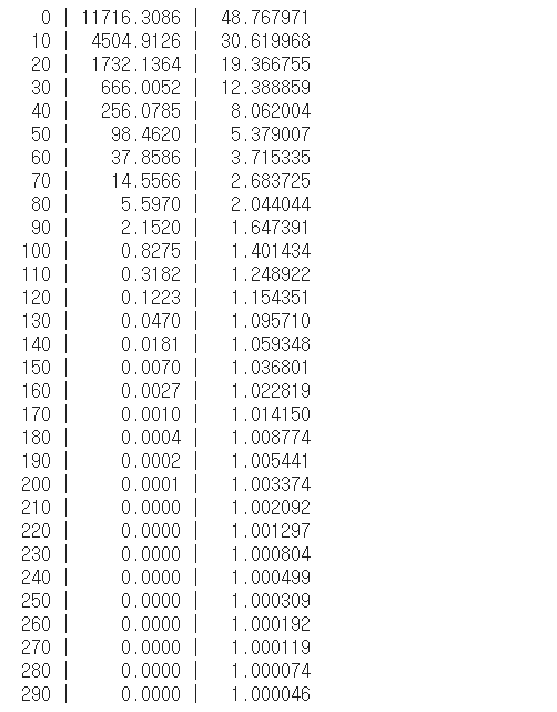

6. Multi-variable Linear Regression

다변수 선형회귀는 다양한 변수를 가지고 예측했을 때 더윽 정확한 예측을 할 수 있다.
Multi-variable = Multi-feature
변수의 개수가 늘어나면 그만큼 가중치의 개수도 늘어난다. → Matrix 활용
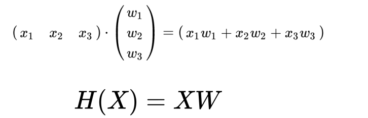matrix는 대문자로 표시
x의 개수, w의 개수에 상관 없이 모든 matrix는 XW로 표현한다.
x_matrix의 column과 w_matrix의 row 개수가 일치해야 dot product가 가능

7. Multi-varialbe LR TensorFlow

import tensorflow as tf
import numpy as np
data = np.array([
    # X1,   X2,    X3,   y
    [ 73.,  80.,  75., 152. ],
    [ 93.,  88.,  93., 185. ],
    [ 89.,  91.,  90., 180. ],
    [ 96.,  98., 100., 196. ],
    [ 73.,  66.,  70., 142. ]
], dtype=np.float32)

#slice data
X = data[:, :-1]
Y = data[:, [-1]]

#랜덤한 초기값으로 x1,x2,x3 변수로 나눠야 하기 때문에 row 3
# 출력값은 하나이기 때문에 wiehgt의 column 1
W = tf.Variable(tf.random.normal((3,1))) 
b= tf.Variable(tf.random.normal((1,)))  # bias 1

learning_rate = 0.000001

# hypothesis, prediction function
def predict(X):
    return tf.matmul(X, W) + b

print("epoch | cost")
n_epochs = 2000
for i in range(n_epochs +1):
  with tf.GradientTape() as tape:
    cost = tf.reduce_mean((tf.square(predict(X))))

    # calculates the gradients of the loss
    W_grad, b_grad = tape.gradient(cost, [W, b])

    # updates parameters (W and b)
    W.assign_sub(learning_rate * W_grad)
    b.assign_sub(learning_rate * b_grad)

    if i % 100 == 0:
        print("{:5} | {:10.4f}".format(i, cost.numpy()))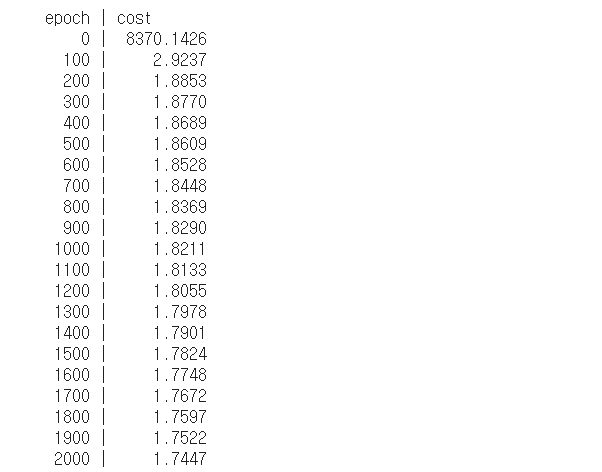

👉 변수의 개수 만큼 써줘야 할 것을 항상 H = WX 동일한 식을 사용하기 때문에 성능면에서 더 유리하다.

8. Logistic Regression/Classification의 cost 함수 최소화

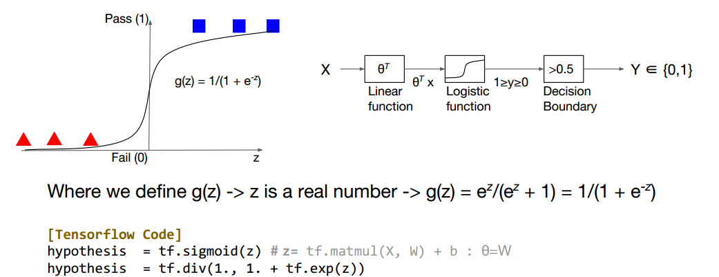Binary classification : 0 or 1 두가지의 값으로 나눈다.
g function을 통해 수치형 값(z)이 sigmoid 함수가 된다.
tensorflow에서 hypothesis = tf.sigmoid(z) ⇒ 1 or 0의 값으로 나타난다.
0<y<1의 값에서 Decision boundary = 0.5로 정했을 때 0.5<y일 때 1, 0.5>y일 때 0이 된다.

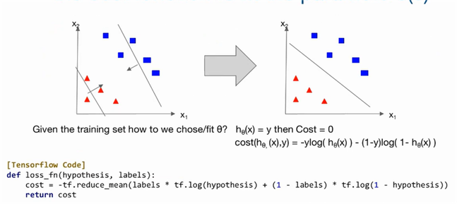labels = y값, hypothesis 가설값
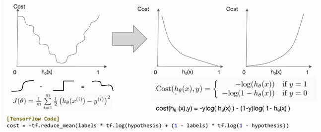J(θ)는 0에 가까워야한다.

9. Logistic Regression/Classification TensorFlow

import numpy as np
import matplotlib.pyplot as plt
%matplotlib inline
import tensorflow as tf

x_train = [[1., 2.],
          [2., 3.],
          [3., 1.],
          [4., 3.],
          [5., 3.],
          [6., 2.]]
y_train = [[0.],
          [0.],
          [0.],
          [1.],
          [1.],
          [1.]]

x_test = [[5.,2.]] 
y_test = [[1.]]
x1 = [x[0] for x in x_train]
x2 = [x[1] for x in x_train]

colors = [int(y[0] % 3) for y in y_train]
plt.scatter(x1,x2, c=colors , marker='^') # scater(): x1, x2의 좌표로 색상을 구분한다. 
plt.scatter(x_test[0][0],x_test[0][1], c="red")

plt.xlabel("x1")
plt.ylabel("x2")
plt.show()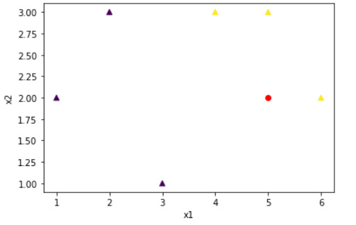

#x_train에 대한 데이터를 가져온다.
dataset = tf.data.Dataset.from_tensor_slices((x_train, y_train)).batch(len(x_train
))
W = tf.Variable(tf.zeros([2,1]), name='weight')
b = tf.Variable(tf.zeros([1]), name='bias')

def logistic_regression(features):
  # tf.exp() = e^(-x)
  hypothesis = tf.divide(1., 1. + tf.exp(tf.matmul(features,W)+b))
  return hypothesis

def loss_fn(hypothesis, features, labels):
  cost = -tf.reduce_mean(labels * tf.math.log(logistic_regression(features)) + (1 - labels) * tf.math.log(1 - hypothesis))
  return cost

optimizer = tf.keras.optimizers.SGD(learning_rate=0.01)

def accuracy_fn(hypothesis, labels):
    predicted = tf.cast(hypothesis > 0.5, dtype=tf.float32)
    accuracy = tf.reduce_mean(tf.cast(tf.equal(predicted, labels), dtype=tf.int32))
    return accuracy

def grad(features, labels):
    with tf.GradientTape() as tape:
        loss_value = loss_fn(logistic_regression(features),features,labels)
    return tape.gradient(loss_value, [W,b])

EPOCHS = 1001

for step in range(EPOCHS):
    for features, labels  in iter(dataset):
        grads = grad(features, labels)
        optimizer.apply_gradients(grads_and_vars=zip(grads,[W,b]))
        if step % 100 == 0:
            print("Iter: {}, Loss: {:.4f}".format(step, loss_fn(logistic_regression(features),features,labels)))
test_acc = accuracy_fn(logistic_regression(x_test),y_test)
print("Testset Accuracy: {:.4f}".format(test_acc))

Iter: 0, Loss: 0.6874
Iter: 100, Loss: 0.5776
Iter: 200, Loss: 0.5349
Iter: 300, Loss: 0.5054
Iter: 400, Loss: 0.4838
Iter: 500, Loss: 0.4671
Iter: 600, Loss: 0.4535
Iter: 700, Loss: 0.4420
Iter: 800, Loss: 0.4319
Iter: 900, Loss: 0.4228
Iter: 1000, Loss: 0.4144
Testset Accuracy: 1.0000