2장 머신러닝 프로젝트 처음부터 끝까지 (1)
2장은 머신러닝 프로젝트 하나를 정하고, 그 문제를 해결해가는 전체 과정을 담고있는 장이다.
1. 준비
- 핸즈온 머신러닝 2: https://tensorflow.blog/handson-ml2
- 깃허브: http://bit.ly/homl2-git
- 슬라이드: http://bit.ly/homl2-slide
- 유튜브: http://bit.ly/homl2-youtube
1-1.캘리포니아 주택 가격 예측
-
인구, 중간 소득 등의 특성(속성? columns?)을 사용하여 중간 주택 가격 예측하는 문제
-
다중 회귀(여러개의 특성), 단변량 회귀-> 하나의 예측 값(반대 : 다변량 회귀)
-
회귀의 성능 측정
-
평균 제곱근 오차
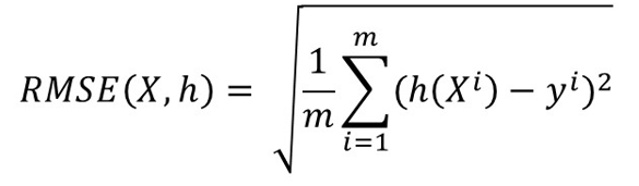
- m : 샘플의 개수
- 모든 샘플에대해 제곱
- x : 특성
- h : 모델이 예측한 값
- y : 타겟값
- 즉, (예측값 - 타겟값)^2 의 모든 값을 더해 m으로 나눠 평균을 구하고, 제곱을 한 값이기 때문에 다시 루트를 씌워주는 의미.
-
평균 절대 오차
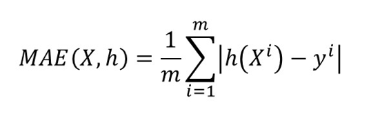
- 위 식과 비슷하지만, 제곱 -> 루트 를 빼고, 음수를 없애기위해 절대값을 사용한 값.
-
1-2.시작하기 전에
표기법
- 소문자(x) : 행렬 스칼라 값, x1 = [경도, 위도, 중간 소득, 주민 ....]
- 소문자(y) : x1에 대한 예측 값, 여기서는 예측된 중간 주택 가격을 뜻한다.
- 대문자(X) : 벡터 값을 이야기 한다., X = [x1, x2, x3.....]
2. 실습
https://github.com/rickiepark/handson-ml2/blob/master/02_end_to_end_machine_learning_project.ipynb
2장 - 머신러닝 프로젝트 처음부터 끝까지 (주피터 노트북)
02_end_to_end_machine_learning_project.ipynb
2-1. 설정
# 파이썬 ≥3.5 필수
import sys
assert sys.version_info >= (3, 5)

# 사이킷런 ≥0.20 필수
import sklearn
assert sklearn.__version__ >= "0.20"

# 공통 모듈 임포트
import numpy as np
import os

# 깔금한 그래프 출력을 위해
# matplotlib inline은 예전 주피터 노트북에서 matplotlib을 사용하기 위한 명령어이다.
%matplotlib inline
import matplotlib as mpl
import matplotlib.pyplot as plt
#글자 크기 크게
mpl.rc('axes', labelsize=14)
mpl.rc('xtick', labelsize=12)
mpl.rc('ytick', labelsize=12)

# 그림을 저장할 위치
PROJECT_ROOT_DIR = "."
CHAPTER_ID = "end_to_end_project"
IMAGES_PATH = os.path.join(PROJECT_ROOT_DIR, "images", CHAPTER_ID)
os.makedirs(IMAGES_PATH, exist_ok=True)

def save_fig(fig_id, tight_layout=True, fig_extension="png", resolution=300):
    path = os.path.join(IMAGES_PATH, fig_id + "." + fig_extension)
    print("그림 저장:", fig_id)
    if tight_layout:
        plt.tight_layout()
    plt.savefig(path, format=fig_extension, dpi=resolution)
2-2. 데이터 가져오기
import os
import tarfile
import urllib.request

DOWNLOAD_ROOT = "https://raw.githubusercontent.com/rickiepark/handson-ml2/master/"
HOUSING_PATH = os.path.join("datasets", "housing")
HOUSING_URL = DOWNLOAD_ROOT + "datasets/housing/housing.tgz"

#다운로드 후 압축 해제 해주는 함수
def fetch_housing_data(housing_url=HOUSING_URL, housing_path=HOUSING_PATH):
    if not os.path.isdir(housing_path):
        os.makedirs(housing_path)
    tgz_path = os.path.join(housing_path, "housing.tgz")
    urllib.request.urlretrieve(housing_url, tgz_path)
    housing_tgz = tarfile.open(tgz_path)
    housing_tgz.extractall(path=housing_path)
    housing_tgz.close()

fetch_housing_data()


import pandas as pd
#CSV파일을 읽고 pandas DataFrame으로 반환해주는 함수
def load_housing_data(housing_path=HOUSING_PATH):
    csv_path = os.path.join(housing_path, "housing.csv")
    return pd.read_csv(csv_path)

housing = load_housing_data()
2-3. 데이터 구조 살펴보기
housing.info()<class 'pandas.core.frame.DataFrame'> RangeIndex: 20640 entries, 0 to 20639 Data columns (total 10 columns): # Column Non-Null Count Dtype --- ------ -------------- ----- 0 longitude 20640 non-null float64 1 latitude 20640 non-null float64 2 housing_median_age 20640 non-null float64 3 total_rooms 20640 non-null float64 4 total_bedrooms 20433 non-null float64 5 population 20640 non-null float64 6 households 20640 non-null float64 7 median_income 20640 non-null float64 8 median_house_value 20640 non-null float64 9 ocean_proximity 20640 non-null object dtypes: float64(9), object(1) memory usage: 1.6+ MB
housing["ocean_proximity"].value_countns()<1H OCEAN 9136 INLAND 6551 NEAR OCEAN 2658 NEAR BAY 2290 ISLAND 5 Name: ocean_proximity, dtype: int64
import matplotlib.pyplot as plt
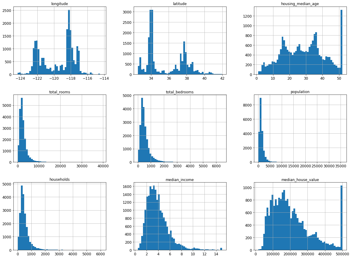
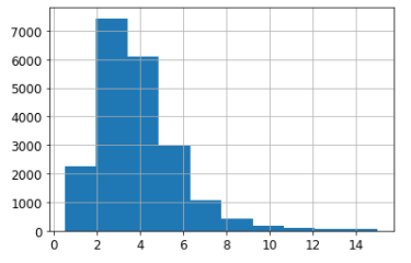
housing.hist(bins=50, figsize=(20, 15))
plt.show()
- 여기서 housing_median_age, housing_median_value 히스토그램을 보면, 제일 오른쪽 그래프에 값이 이상하게 큰 것을 볼 수 있다.
- 이는, 최대값으로 일정값 이상이면 모두 포함한 그래프라고 추측할 수 있다. 즉, 이 데이터를 사용한다면 그 일정값 이상의 예측은 정확하지 않을 것이다.
- 이럴때는 그 값을 제거한다거나, 일정값 이상의 데이터를 새로 수집하는 방법으로 해결 할 수 있다.
- 또한, 대부분의 그래프가 왼쪽으로 치우쳐져있다. 흔히 가우시안 모양이라고 하는 종 모양에 가깝게, 표준형에 가깝게 만드는 법도 다룰 것이다.
- 데이터의 스케일도 각각 다른데, 데이터의 단위가 다를때, 이 스케일을 맞추는 방법도 살펴볼것이다.
2-4. 테스트 세트 만들기1
훈련데이터로 훈련 후, 테스트세트로 평가할 때, 테스트세트가 모델을 훈련하는데에 기여를 한다면, 테스트 세트가 평가를 공정하게 하지 못 할 수 있다. 따라서, 미리 테스트 세트를 떨어뜨려 놔야 한다.
sklearn.model_selection의 train_test_split을 사용하는 코드 (대부분 이 방법을 사용한다.)
#주피터 노트북의 실행 결과가 동일하도록
from sklearn.model_selection import train_test_split
train_set, test_set = train_test_split(housing, test_size=0.2, random_state=42)
print(len(train_set))  # 16512
print(len(test_set))	# 4128
Sklearn.model_selction의 train_test_split을 함수로 만들어본 코드
import numpy as np
# 예시로 만든 것입니다. 실전에서는 사이킷런의 train_test_split()를 사용하세요.
def split_train_test(data, test_ratio):
  #np.random.permutation : 배열을 입력하면 배열을 섞어주고, 정수를 입력하면, 0~정수까지의 배열을 만든 후, 섞어저 리턴해준다.
    shuffled_indices = np.random.permutation(len(data))
    test_set_size = int(len(data) * test_ratio)
    test_indices = shuffled_indices[:test_set_size]
    train_indices = shuffled_indices[test_set_size:]
    return data.iloc[train_indices], data.iloc[test_indices
train_set, test_set = split_train_test(housing, 0.2)
print(len(train_set))  # 16512
print(len(test_set))	# 4128
TEST셋을 섞이지 않게 crc32 체크섬을 이용하여 고정해서 사용하는 방법
- 각 샘플마다 고유한 아이디가 있다면 그것을 해싱해서, 해싱값이 일정값 이하일 때, test으로 사용하는 방법
- crc32 체크썸을 사용한다.
  #정수의 범위에 해당하는 값으로 바꿈. -> 체크썸
  # 그중에 test_ratio * 2**32 보다 작은건 test, 더 크면 train
  # 오른쪽처럼 비트연산을 하는 이유는, crc32가 python2에서는 양수만 나오지만, python3에서는 음수도 나올 수 있기 때문에
  #python document에서 권장하는 방법이다.
  #참고로 and연산 0xfffffff는 앞자리수를 0으로 만들고 나머지만 나오게 하는 방법같다.
from zlib import crc32
def test_set_check(identifier, test_ratio):
	return crc32(np.int64(identifier)) & 0xffffffff < test_ratio * 2**32
#만약 데이터가 DateFrame일 때, data[id_columns]을 뽑는다. #그러면 Series가 될텐데, 그 시리즈에 lambda함수로 test_set_check를 통과시킨다. #그렇다면 과연 이 id가 crc32 체크섬에서 나온 값이 test_ratio보다 작냐 크냐 확인한 후, train셋과 test셋을 다시 구분해주는 함수이다. def split_train_test_by_id(data, test_ratio, id_column): ids = data[id_column] in_test_set = ids.apply(lambda id_: test_set_check(id_, test_ratio)) return data.loc[~in_test_set], data.loc[in_test_set]housing_with_id = housing.reset_index() # `index` 열이 추가된 데이터프레임을 반환합니다 train_set, test_set = split_train_test_by_id(housing_with_id, 0.2, "index") print(len(train_set)) # 16512 print(len(test_set)) # 4128
2-5. 테스트 세트 만들기 2
범주형 데이터로 변환
housing["median_income"].hist()
- median_income (중간소득)이 매우 중요한 데이터라면, 데이터가 고르게 분포되어 있을수록 좋은 결과를 얻을 수 있다.
- 각 test셋과 train데이터에 고르게 분포되어 있어야 좋다. 따라서 레벨별, 수준별로 나눠 범주형 데이터로 바꿔 고르게 나눌 것이다.
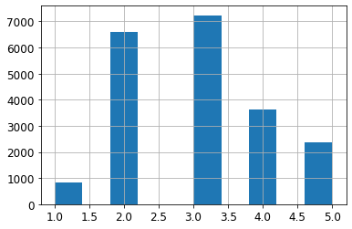
housing["income_cat"] = pd.cut(housing["median_income"], bins=[0., 1.5, 3.0, 4.5, 6., np.inf], lavels=[1, 2, 3, 4, 5])
housing["income_cat"].value_counts()3 7236 2 6581 4 3639 5 2362 1 822 Name: income_cat, dtype: int64
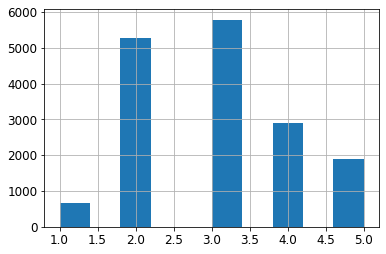
housing["income_cat"].hist()
sklearn.model_selection의 stratifiedShuffleSplit 사용하기
from sklearn.model_selection import StratifiedShuffleSplit
split = StratifiedShuffleSplit(n_splits=1, test_size=0.2, random_state=42)   #n_split: train, test로만 나눌것이기 때문에 1
for train_index, test_index in split.split(housing, housing["income_cat"]):  #분배할 DataFrame, 그중에서 분배할 Columns
    strat_train_set = housing.loc[train_index]    # n_split == 1 이기때문에 for문은 한번만 돌아갈 것이다.
    strat_test_set = housing.loc[test_index]
- sklearn에서 Stratified가 붙으면, 계층형 분할이라 생각 할 수 있다. (범주형 분할)
- 분할결과 strat_test_set과 원본 housing 둘다 value_counts는 같은 값이 나온다.
start_test_set["income_cat"].value_counts()/len(strat_test_set)3 0.350533 2 0.318798 4 0.176357 5 0.114341 1 0.039971 Name: income_cat, dtype: float64
housing["income_cat"].value_counts()/len(housing)3 0.350581 2 0.318847 4 0.176308 5 0.114438 1 0.039826 Name: income_cat, dtype: float64
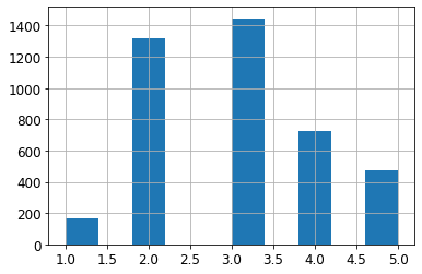
- 그러나 strat_test_set["income_cat"]은 그래프로 그리면 잘 분포된 것을 볼 수 있다.
strat_test_set["income_cat"].hist()
sklearn.model_slection의 train_test_split 사용하기
- sklearn.model_selection의 train_test_split모듈에서도 train, test셋 분리와 동시에 분포형으로 나눠줄 수 있다.
st_train_set, st_test_set = train_test_split(housing, test_size=0.2, random_state=42, **stratify=housing["income_cat"]**)3 0.350594 2 0.318859 4 0.176296 5 0.114462 1 0.039789 Name: income_cat, dtype: float64