https://yamalab.tistory.com/132?category=747907
벡터간의 유사도 계산은 엄청난게 오래걸리고, 이를 실시간으로 처리하기에는 너무 오래걸린다
대신에 k-Nearest Neighbor를 찾기 위한 별도의 벡터 색인 작업이 필요하다!
-
벡터를 색인한다는 것은 유사 벡터를 빠르게 찾을 수 있는 데이터 구조를 구축하는 것을 의미
-
해싱 기반의 방법
- 이 방법은 Elasticsearch 같은 검색 엔진(7 버전 이상에서 제공하는 densed vector similarity 기능), 혹은 Annoy같은 라이브러리에서 주로 사용되는 방법이다.
- 해싱 방법에는 LSH, PCA 해싱 등 여러 가지 방법이 있다
- 역색인을 활용 예제
- 만약 [x1, x2, x3, x4...] 으로 이루어진 벡터의 각 요소를 x1 mod M 같은 아주 간단한 해싱 알고리즘으로 매핑했다고 가정하자(해싱 테이블의 크기는 M). 그러면 xn 요소는 임의의 해시값으로 매핑이 되었을 것이고, [a, b, a, c..] 와 같은 결과가 되었을 것이다(a,b,c...M). 이제 역색인 구조로 이것을 다시 살펴본다면, a라는 해싱값을 가지고 있는 벡터 리스트 [v1, v2..], b라는 해싱값을 가지고 있는 벡터 리스트 [v2, v4..]와 같은 인덱스 형태가 될 것이다. 이 구조를 활용하면 유사한 벡터들의 subset을 줄여나가는 방식으로 효율적인 kNN 검색을 할 수 있게 된다.
- Annoy 같은 라이브러리에서 사용되는 Random Projection 기반의 알고리즘 예제
- Random Projection은 고차원 벡터를 저차원 벡터로 매핑하는 차원 축소의 개념이다.
- PCA 혹은 t-SNE 같은 대표적인 벡터 축소 방식과 개념 자체(원래의 행렬을 재현할 수 있는 Middle Factor가 존재한다는 개념)는 거의 유사하다.
- 단, Random Projection은 Johnson-Linderstrauss Lemma의 수식을 이용하여 N차원이면서 k개의 Point를 가지고있는 벡터를 특정 차원 M으로 매핑해주는 함수를 알고 있다는 것이 다르다. 자세한 내용은 링크의 블로그에서 훌륭하게 설명되어 있으니 참고하자. 어쨌든 이러한 차원 축소 방법을 이용해서, 벡터를 Bucketizing 한 뒤에 이를 Search Space로 활용한다. 이때, 원래의 벡터를 특정한 Space로 편입시키는 과정을 Locality Sensitve Hashing이라고 한다.
-
트리 기반의 방법
- 트리 기반의 접근법은 divide and conquer 아이디어에서 떠올린 것이라고 할 수 있다.
- 어떻게든 트리 형태로 vector point를 배치하여, O(log n) 시간 안에 인접한 벡터를 찾겠다는 목표를 가지고 만들어진 형태이다. 하지만 아마도 짐작할 수 있듯이, 모든 데이터를 트리에 넣어야 하므로 상대적으로 많은 메모리를 사용하게 된다. 또한 divide 성능에 따라 search의 성능이 매우 크게 좌우될 수 있다는 단점도 있다.
- 이에 대한 한 가지 예로 트리 기반의 ANNS중 가장 대표적인 kd-tree(K-Dimension Tree)를 간단히 살펴보자. kd-tree는 간단하게는 binary search tree를 다차원 공간으로 확장한 것이라고 할 수 있다. 다만 다른 점은 트리의 레벨 차원을 번갈아가며 비교한다는 것이다.
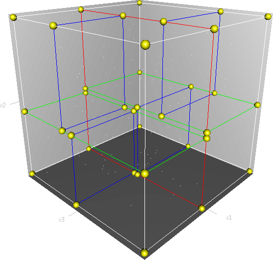
- 공간을 분할하는 검색 방식인 kd-tree
- 예를 들어 3개의 축을 가진 데이터라고 하면, 위의 그림처럼 하나의 축으로 부피를 분할하고, 나머지 두개의 축 레벨에서 부피를 분할하는 식으로 반복 분할한다. 먼저 X축을 기준으로 YZ 평면을 분할하고, 다음으로 Y축을 기준으로 XZ 평면을 분할, 그리고 Z축을 기준으로 XY 평면을 분할하는 식이라고 이해하면 좋다. 일반적인 BST의 프랙탈 버전이라고 할 수 있겠다.
-
네트워크 기반의 방법
-
Network based NN indexer
https://lovit.github.io/machine learning/vector indexing/2018/09/10/network_based_nearest_neighbors/
-
Scaling nearest neighbors search with approximate methods
https://www.jeremyjordan.me/scaling-nearest-neighbors-search-with-approximate-methods/
-
intro
- The process of finding vectors that are close to our query is known as nearest neighbors search.
- 나이브하게는 calculate the distance between the query vector and every vector in our collection (commonly referred to as the reference set) 로 생각할 수 있지만, 너무 오래걸림ㅠ
- A class of methods known as approximate nearest neighbors search offer a solution to our scaling dilemma by partitioning the vector space in a clever way such that we only need to examine a small subset of the overall reference set.
-
Tree-based data structures
-
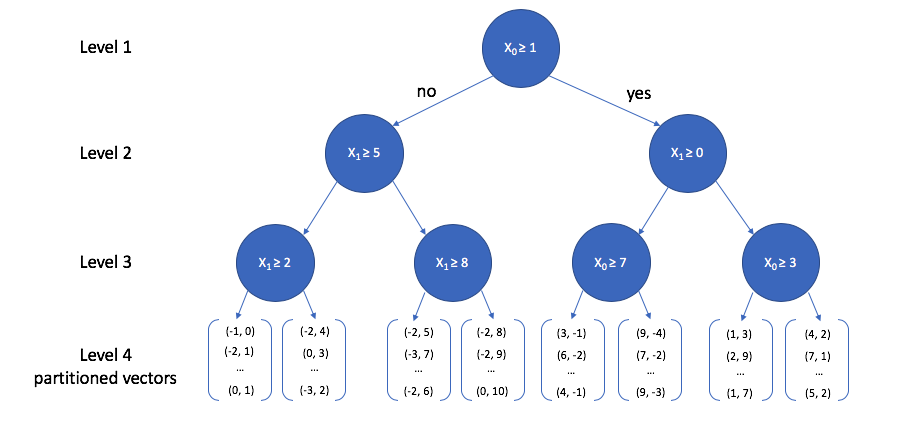
K-dimensional trees
: K-dimensional trees 는 binary search 트리의 컨셉을 다차원으로 일반화 한 것
- The general procedure for growing a k-dimensional tree is as follows:
- pick a random dimension from your k-dimensional vector
- find the median of that dimension across all of the vectors in your current collection
- split the vectors on the median value
- repeat!
- k-차 벡터에서 random dimension을 하나 택한다
- 현재 우리가 갖고 있는 collection(reference set: 쉽게 말해, 내가 가진 모든 벡터들의 집합)에서, 모든 벡터들을 가로질러서 방금 선택한 dimention의 중앙값을 찾는다.
- 중앙값에 대해 벡터를 나눈다
- 반복!
A toy 2-dimensional example is visualized below.
- At the top level, we select a random dimension (out of the two possible dimensions, x0 and x1)
- calculate the median.
- Then, we follow the same procedure of picking a dimension and calculating the median for each path independently.
- This process is repeated until some stopping criterion is satisfied; each leaf node in the tree contains a subset of vectors from our reference set.
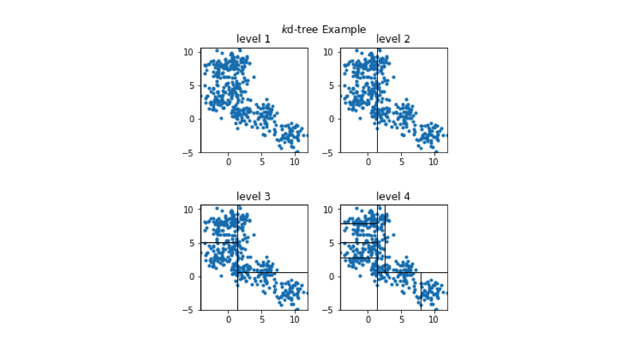
We can view how the two-dimensional vectors are partitioned at each level of the k-d tree in the figure below.
-
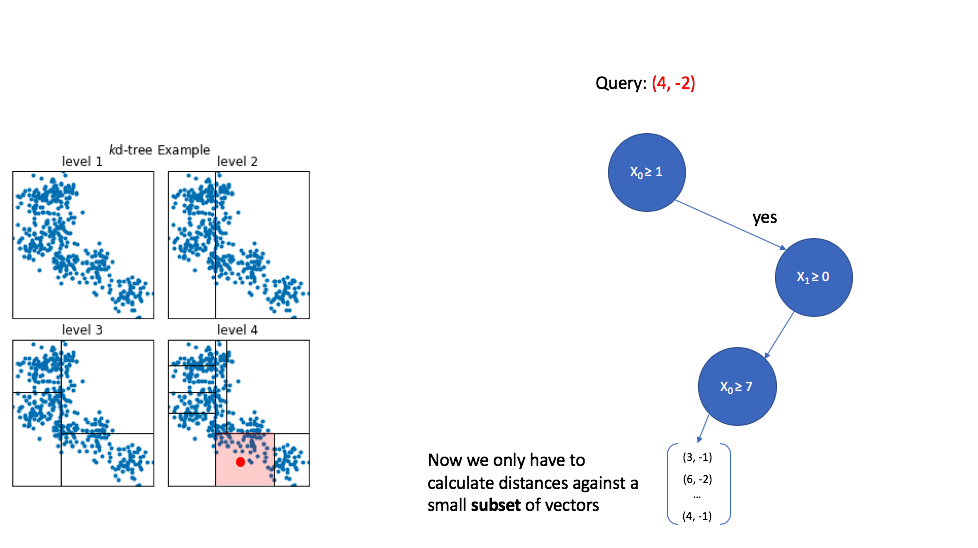
In order to see the usefulness of this tree,
let's now consider how we could use this data structure to perform an approximate nearest neighbor query. As we walk down the tree, notice how the highlighted area (the area in vector space that we're interested in) shrinks down to a small subset of the original space. (I'll use the level 4 subplot for this example.)
→ K-d trees are popular due to their simplicity, however, this technique struggles to perform well when dealing with high dimensional data.
→ 지금까지의 예시는 나뉘어진 cell의 중간에 위치했을 경우를 살펴보고 있지만, cell의 경계에 위치하였을 때는 어떻게 해야할까? we miss out on vectors which lie just outside of the cell.
- The general procedure for growing a k-dimensional tree is as follows:
-
Quantization
- 우리의 reference set을 잘게 나눠서, 더 작은 collection of representative vectors으로 만드는게 우리의 목적이다.
- We can find these "representative" vectors by simply running the K-means algorithm on our data.
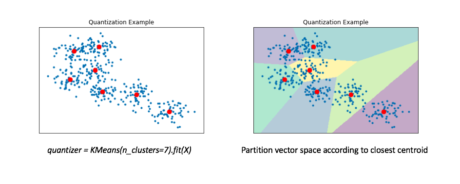
- The right figure displays a Voronoi diagram which essentially partitions the space according to the set of points for which a given centroid is closest.
- We'll then "map" all of our data onto these centroids.
- we can represent our reference set of a couple hundred vectors with only 7 representative centroids.
- This greatly reduces the number of distance computations we need to perform (only 7!) when making an nearest neighbors query.
We can then maintain an inverted list to keep track of all of the original objects in relation to which centroid represents the quantized vector.
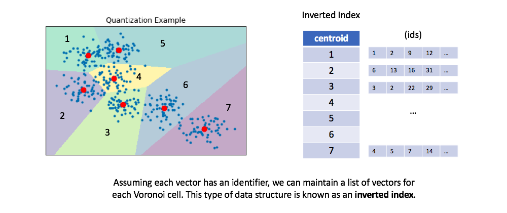
- You can optionally retrieve the full vectors for all of the ids maintained in the inverted list for a given centroid, calculating the true distances between each vector and our query.
- This is a process known as re-ranking and can improve your query performance.
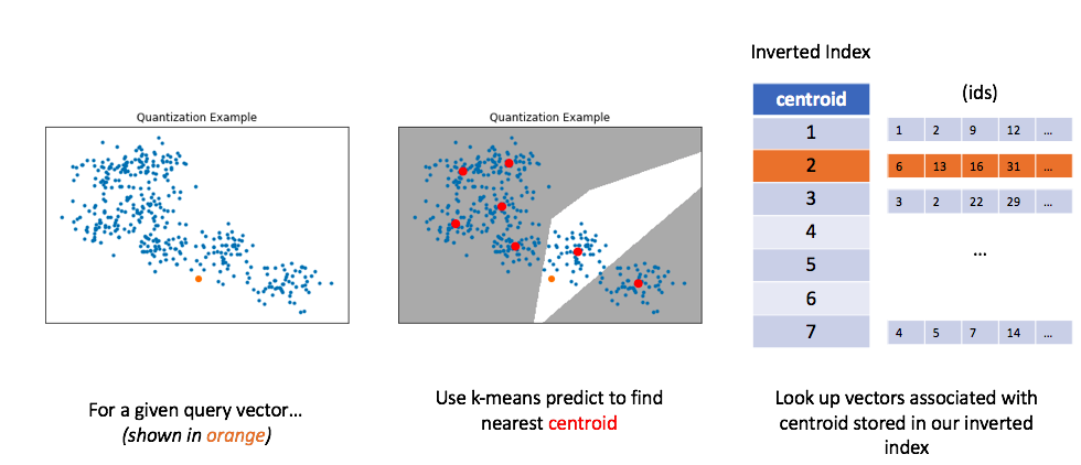
Similar to before, let's now look at how we can use this method to perform a query. For a given query vector, we'll calculate the distances between the query vector and each centroid in order to find the closest centroid. We can then look up the centroid in our inverted list in order to find all of the nearest vectors.
Unfortunately, in order to get good performance using quantization, you typically need to use very large numbers of centroids for quantization; this impedes on original goal of alleviating the computational burden of calculating too many distances.
-
Product quantization
-
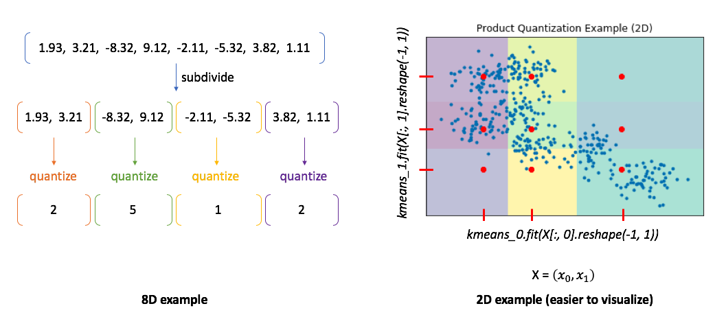
Product quantization는 문제를 이렇게 풀어낸다 by first subdividing the original vectors into subcomponents and then quantizing (ie. running K-means on) each subcomponent separately.
-
A single vector is now represented by a collection of centroids, one for each subcomponent.
-
examples:
→ In the 8D case, you can see how our vector is divided into subcomponents and each subcomponent is represented by some centroid value.
→ However, the 2D example shows us the benefit of this approach. In this case, we can only split our 2D vector into a maximum of two components.
We'll then quantize each dimension separately, squashing all of the data onto the horizontal axis and running k-means and then squashing all of the data onto the vertical axis and running k-means again.
We find 3 centroids for each subcomponent with a total of 6 centroids. However, the total set of all possible quantized states for the overall vector is the Cartesian product of the subcomponent centroids.
-
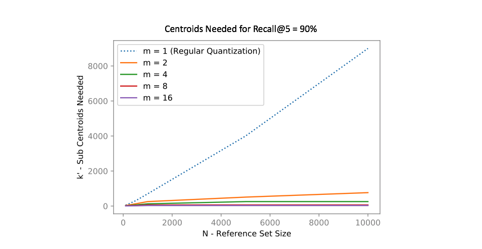
In other words, if we divide our vector into m subcomponents and find k centroids, we can represent k^m possible quantizations using only km vectors! The chart below shows how many centroids are needed in order to get 90% of the top 5 search results correct for an approximate nearest neighbors query.
→ represent 3^2 quantization using 3*2 vectors
-
Notice how using product quantization (m>1m>1) vastly reduces the number of centroids needed to represent our data. One of the reasons why I love this idea so much is that we've effectively turned the curse of dimensionality into something highly beneficial!
-
-
Handling multi-modal data
-
Product quantization 는 데이터가 벡터공간에 고르게 퍼져있을 때 잘 작동한다
-
However, in reality our data is usually multi-modal.
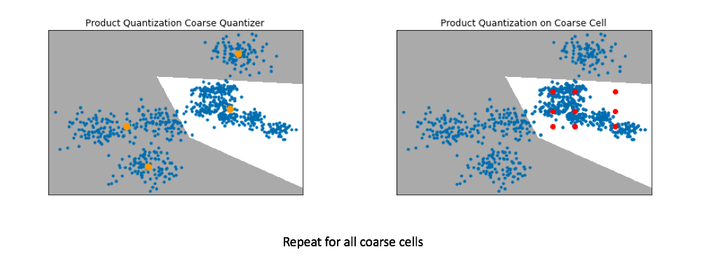
→ To handle this, a common technique involves first training a coarse quantizer to roughly "slice" up the vector-space, and then we'll run product quantization on each individual coarse cell.
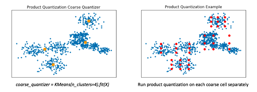
- Below, I've visualized the data that falls within a single coarse cell. We'll use product quantization to find a set of centroids which describe this local subset of data, and then repeat for each coarse cell.
- Commonly, people encode the vector residuals (the difference between the original vector and the closest coarse centroid) since the residuals tend to have smaller magnitudes and thus lead to less lossy compression when running product quantization. In simple terms, we treat each coarse centroid as a local origin and run product quantization on the data with respect to the local origin rather than the global origin.
Pro-tip: If you want to scale to really large datasets you can use product quantization as both the coarse quantizer and the fine-grained quantizer within each coarse cell. See this paper for the details.
-
-
Locally optimized product quantization
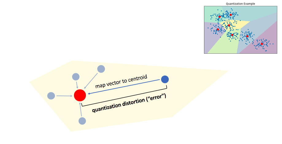
The ideal goal for quantization is to develop a codebook which is (1) concise and (2) highly representative of our data. More specifically, we'd like all of the vectors in our codebook to represent dense regions of our data in vector-space. A centroid in a low-density area of our data is inefficient at representing data and introduces high distortion error for any vectors which fall in its Voronoi cell.
One potential way we can attempt to avoid these inefficient centroids is to add an alignment step to our product quantization. This allows for our product quantizers to better cover the local data for each coarse Voronoi cell.
We can do this by applying a transformation to our data such that we minimize our quantization distortion error. One simple way to minimize this quantization distortion error is to simply apply PCA in order to mean-center the data and rotate it such that the axes capture most of the variance within the data.
Recall my earlier example where we ran product quantization on a toy 2D dataset. In doing so, we effectively squashed all of the data onto the horizontal axis and ran k-means and then repeated this for the vertical axis. By rotating the data such that the axes capture most of the variance, we can more effectively cover our data when using product quantization.
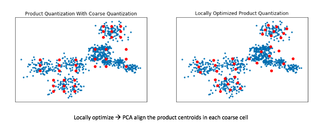
This technique is known as locally optimized product quantization, since we're manipulating the local data within each coarse Voronoi cell in order to optimize the product quantization performance. The authors who introduced this technique have a great illustrative example of how this technique can better fit a given set of vectors.
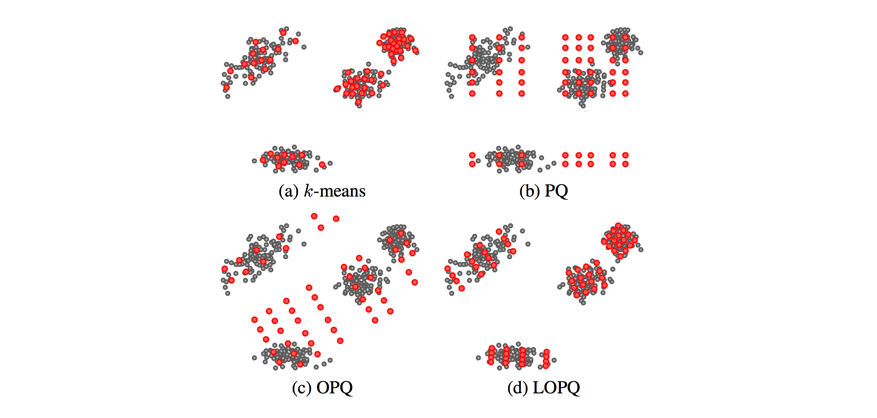
This blog post glances over (c) Optimized Product Quantization which is the same idea of aligning our data for better product quantization performance, but the alignment is performed globally instead of aligning local data in each Voronoi cell independently. Image credit
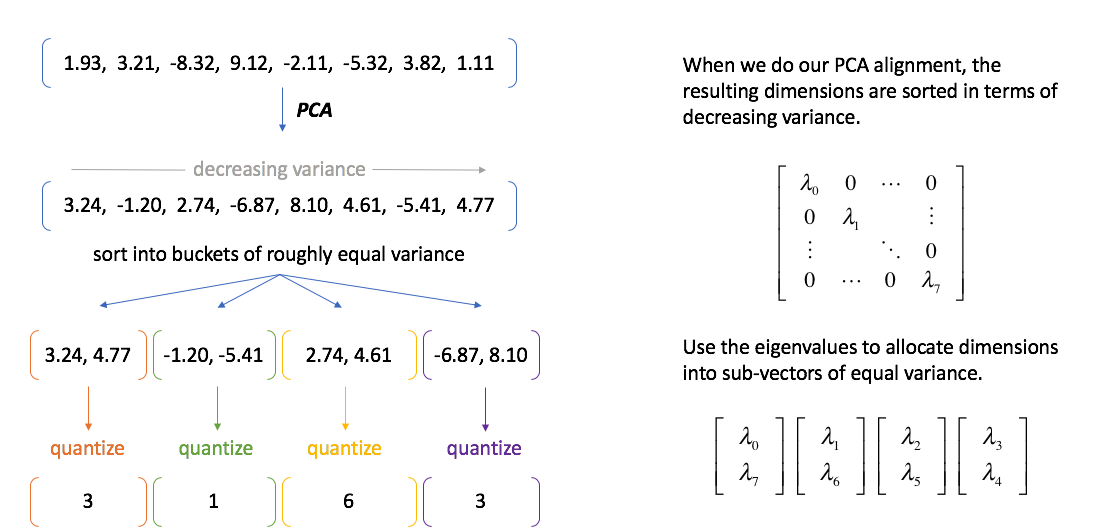
A quick sidenote regarding PCA alignment
The authors who introduced product quantization noted that the technique works best when the vector subcomponents had similar variance. A nice side effect of doing PCA alignment is that during the process we get a matrix of eigenvalues which describe the variance of each principal component. We can use this to our advantage by allocating principal components into buckets of equal variance.
-
-
-
spotify/ annoy
Vector Search
-
Vector Search는 point가 매우 많아지면 곤란한 상황이 된다.
-
그래서 Approximated 계산이 필요해진다.
-
기본적인 아이디어는 벡터를 공간상에 분리하거나, 해싱 트릭으로 Bucketizing 하는 것이다. 어쨌든 데이터를 큰 그룹으로 나눠놓는 게 목표가 된다.
-
결국 특정 벡터와 가까운 벡터를 찾으려면, 그룹 내 벡터들과의 거리만 계산하면 된다.
-
이걸 Real-time으로 활용하기 위해 색인 과정까지 거치면 된다. 검색이니까 역색인을 활용하면 더 좋다. 비유하자면 학생들한테 "너랑 가장 친한 친구가 누구인지 물어볼테니까 미리 결정해놔" 같은 작업이다.
-
Happy Searching!