
사용자는 실행 계획을 분석함으로써 쿼리 복잡성을 파악하여 간소화하고 런타임을 개선할 수 있습니다. 실행 전에 EXPLAIN 명령문을 사용하여 SQL 구문의 유효성을 검사할 수도 있는데, 이렇게 하면 실행 중에 발생할 수 있는 오류를 방지하는 데 도움이 됩니다.
EXPLAIN을 사용하는 방식은 presto에서도 동일하게 사용 가능합니다. 하지만 presto의 경우 다양한 데이터 소스 위에서 동작하는 분산 처리 SQL엔진이므로 다른 데이터베이스에서의 실행 계획과 다소 다릅니다. presto의 동작방식을 이해하고 결과를 해석하려고 한 부분에 대해서 공유하려고 합니다.
Presto란?
Presto는 Facebook 개발자가 여러 데이터 소스에서 대량의 데이터에 대해 대화형 분석을 실행하기 위해 만든 오픈소스 분산 SQL 쿼리 엔진입니다. Presto는 모든 데이터 분석 및 개방형 레이크하우스를 위한 하나의 간단한 ANSI SQL 인터페이스를 제공하는 빠르고 안정적인 엔진입니다.
Presto를 왜 사용하는가?
- One Language
- One Interface
- Fast, Reliable & Efficient
자세한 설명은 주제와 멀어질 수 있으므로 https://prestodb.io/what-is-presto.html#why_presto 를 참조하시기 바랍니다.
Presto 작동 방식
실행 계획을 이해하기 위해 presto의 작동 방식을 먼저 이해해야합니다.
Presto는 하나의 Coordinator와 다수의 Worker로 구성되어 있습니다.
- Coordinator : 쿼리 요청을 받아 계획을 세우고 계획을 최적화하고 스케쥴링하는 역할을 한다. Metadata, Data Location API는 쿼리 계획 수립/최적화에 활용한다.
- Worker : Coordinator가 할당한 Task를 수행한다. Data Source API는 데이터 로드 작업에 사용한다.
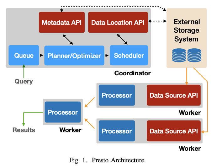
출처 : Presto_SQL_on_Everything
- 쿼리 구문 분석 및 최적화: SQL 쿼리가 Presto에 제출되면 coordinator는 먼저 구문 분석 및 분산 실행 계획 생성 및 최적화를 통해 요청을 처리합니다. 이 계획은 쿼리할 데이터 원본, 필터링할 데이터 및 수행할 계산을 포함하여 쿼리를 실행하는 데 필요한 다양한 stage를 지정합니다.
- 쿼리 조정: coordinator는 각 stage에 task를 worker들에게 할당하고 worker들간의 데이터 교환을 조정합니다.
- 분산 쿼리 실행: worker는 coordinator로부터 쿼리 실행 계획의 일부를 받고 자신이 담당하는 데이터 소스에서 계획을 실행합니다. 각 worker는 다른 worker와 병렬로 쿼리의 일부를 처리하고 필요에 따라 coordinator 및 다른 worker와 데이터를 교환합니다.
- 결과 집계: worker가 쿼리의 일부를 완료하면 결과를 coordinator에게 다시 보내고 coordinator는 결과를 집계하여 사용자에게 반환합니다.
Presto EXPLAIN
EXPLAIN [ ( option [, ...] ) ] statementoption
FORMAT { TEXT | GRAPHVIZ | JSON }
TYPE { LOGICAL | DISTRIBUTED | VALIDATE | IO }
명령문의 logical 또는 distributed execution plan을 표시하거나 명령문의 validate를 검사합니다. fragmented plan을 보려면 TYPE DISTRIBUTED 옵션을 사용하십시오.
Logical plan
presto:tiny> EXPLAIN SELECT regionkey, count(*) FROM nation GROUP BY 1;
                                                Query Plan
----------------------------------------------------------------------------------------------------------
 - Output[regionkey, _col1] => [regionkey:bigint, count:bigint]
         _col1 := count
     - RemoteExchange[GATHER] => regionkey:bigint, count:bigint
         - Aggregate(FINAL)[regionkey] => [regionkey:bigint, count:bigint]
                count := "count"("count_8")
             - LocalExchange[HASH][$hashvalue] ("regionkey") => regionkey:bigint, count_8:bigint, $hashvalue:bigint
                 - RemoteExchange[REPARTITION][$hashvalue_9] => regionkey:bigint, count_8:bigint, $hashvalue_9:bigint
                     - Project[] => [regionkey:bigint, count_8:bigint, $hashvalue_10:bigint]
                             $hashvalue_10 := "combine_hash"(BIGINT '0', COALESCE("$operator$hash_code"("regionkey"), 0))
                         - Aggregate(PARTIAL)[regionkey] => [regionkey:bigint, count_8:bigint]
                                 count_8 := "count"(*)
                             - TableScan[tpch:tpch:nation:sf0.1, originalConstraint = true] => [regionkey:bigint]
                                     regionkey := tpch:regionkey
Logical Plan을 읽는 방법.
- 일반적으로 표현되는 tree 구조에서 tree의 꼭대기에서 아래로 내려가면서 각 operator를 차례로 검사.
- 화살표는 operator 간의 데이터 흐름을 나타냅니다.
- operator 이해 (아래 참조)
Exchange: worker noder간에 데이터가 교환되는 방식. local or remote
-
LocalExchange [exchange_type]: 쿼리의 여러 단계에 대해 작업자 노드 내에서 로컬로 데이터를 전송합니다.
-
RemoteExchange [exchange_type]: 쿼리의 여러 단계에 대해 작업자 노드 간에 데이터를 전송합니다.
-
Exchange types
-
Logical Exchange types
- GATHER: 하나의 worker node가 다른 모든 worker node로부터 output을 수집합니다.
- REPARTITION: 다음 operator에 적용하는 데 필요한 partitioning schema를 기반으로 특정 worker에게 row data를 보냅니다.
- REPLICATE: row data를 모든 worker에게 복사합니다.
-
Distributed Exchange types
- HASH: 해시 함수를 사용하여 여러 대상에 데이터를 배포합니다.
- SINGLE: 하나의 대상에 데이터를 배포합니다.
-
Project : 테이블에서 선택한 column과 변환된 값을 사용하여 다음 추가 처리를 위해 다음 operator로 전달할 수 있습니다.
SCAN: data를 스캔하는 방식
- TableScan: table의 source data를 scan.
- ScanFilter: source data를 scan하고 filter 조건자 및 partition pruning
- ScanFilterProject: source data를 scan하고 filter 조건자 및 partition pruning. output 데이터의 memory 레이아웃을 새로운 projection으로 수정하여 후속 단계의 성능을 향상
Distributed plan
presto:tiny> EXPLAIN (TYPE DISTRIBUTED) SELECT regionkey, count(*) FROM nation GROUP BY 1;
                                          Query Plan
----------------------------------------------------------------------------------------------
 Fragment 0 [SINGLE]
     Output layout: [regionkey, count]
     Output partitioning: SINGLE []
     - Output[regionkey, _col1] => [regionkey:bigint, count:bigint]
             _col1 := count
         - RemoteSource[1] => [regionkey:bigint, count:bigint]

 Fragment 1 [HASH]
     Output layout: [regionkey, count]
     Output partitioning: SINGLE []
     - Aggregate(FINAL)[regionkey] => [regionkey:bigint, count:bigint]
             count := "count"("count_8")
         - LocalExchange[HASH][$hashvalue] ("regionkey") => regionkey:bigint, count_8:bigint, $hashvalue:bigint
             - RemoteSource[2] => [regionkey:bigint, count_8:bigint, $hashvalue_9:bigint]

 Fragment 2 [SOURCE]
     Output layout: [regionkey, count_8, $hashvalue_10]
     Output partitioning: HASH [regionkey][$hashvalue_10]
     - Project[] => [regionkey:bigint, count_8:bigint, $hashvalue_10:bigint]
             $hashvalue_10 := "combine_hash"(BIGINT '0', COALESCE("$operator$hash_code"("regionkey"), 0))
         - Aggregate(PARTIAL)[regionkey] => [regionkey:bigint, count_8:bigint]
                 count_8 := "count"(*)
             - TableScan[tpch:tpch:nation:sf0.1, originalConstraint = true] => [regionkey:bigint]
                     regionkey := tpch:regionkey
Distributed Plan을 읽는 방법.
- Source 및 Sink node 찾기
- source node: 테이블 또는 다른 데이터 소스에서 데이터를 읽는 쿼리의 시작점
- sink node: 결과가 수집되어 사용자에게 반환되는 쿼리의 마지막 단계입니다.
- 다양한 유형의 노드 식별: Distributed Plan의 노드는 데이터에 대해 filter, sort, aggregate 또는 join과 같은 다양한 작업을 수행할 수 있습니다. 각 유형의 노드에는 특정 목적이 있으며 쿼리가 처리되는 방식을 이해하는 데 도움이 될 수 있습니다.
- data flow를 따라가기
- 데이터가 한 단계에서 다음 단계로 이동함에 따라 partitioned, shuffled 또는 다른 노드로 broadcasted 될 수 있습니다. 데이터 흐름을 따라가면 쿼리가 병렬화되고 성능을 위해 최적화되는 방식을 이해하는 데 도움이 됩니다.
fragment type은 Presto node에서 fragment가 실행되는 방식과 fragment 간에 배포되는 방식을 지정합니다.
- SINGLE : Fragment가 single node에서 실행됩니다.
- HASH : hash function을 사용하여 배포된 입력 데이터로 고정된 수의 노드에서 실행됩니다.
- ROUND_ROBIN : round robin 방식으로 배포된 입력 데이터로 고정된 수의 노드에서 실행됩니다.
- BROADCAST : 고정된 수의 노드에서 실행되며 입력 데이터는 모든 노드에 브로드캐스트됩니다.
- SOURCE : 입력 분할에 액세스되는 노드에서 실행됩니다.
Validate
presto:tiny> EXPLAIN (TYPE VALIDATE) SELECT regionkey, count(*) FROM nation GROUP BY 1;
 Valid
-------
 true
IO
presto:hive> EXPLAIN (TYPE IO, FORMAT JSON) INSERT INTO test_nation SELECT * FROM nation WHERE regionkey = 2;
            Query Plan
-----------------------------------
 {
   "inputTableColumnInfos" : [ {
     "table" : {
       "catalog" : "hive",
       "schemaTable" : {
         "schema" : "tpch",
         "table" : "nation"
       }
     },
     "columns" : [ {
       "columnName" : "regionkey",
       "type" : "bigint",
       "domain" : {
         "nullsAllowed" : false,
         "ranges" : [ {
           "low" : {
             "value" : "2",
             "bound" : "EXACTLY"
           },
           "high" : {
             "value" : "2",
             "bound" : "EXACTLY"
           }
         } ]
       }
     } ]
   } ],
   "outputTable" : {
     "catalog" : "hive",
     "schemaTable" : {
       "schema" : "tpch",
       "table" : "test_nation"
     }
   }
 }
Presto EXPLAIN ANALYZE
EXPLAIN ANALYZE [VERBOSE] statement각 작업의 수행시간이나 데이터 크기까지 알고 싶으면 EXPLAIN ANALYZE 를 사용하면 됩니다.
presto:sf1> EXPLAIN ANALYZE SELECT count(*), clerk FROM orders WHERE orderdate > date '1995-01-01' GROUP BY clerk;

                                          Query Plan
-----------------------------------------------------------------------------------------------
Fragment 1 [HASH]
    Cost: CPU 88.57ms, Input: 4000 rows (148.44kB), Output: 1000 rows (28.32kB)
    Output layout: [count, clerk]
    Output partitioning: SINGLE []
    - Project[] => [count:bigint, clerk:varchar(15)]
            Cost: 26.24%, Input: 1000 rows (37.11kB), Output: 1000 rows (28.32kB), Filtered: 0.00%
            Input avg.: 62.50 lines, Input std.dev.: 14.77%
        - Aggregate(FINAL)[clerk][$hashvalue] => [clerk:varchar(15), $hashvalue:bigint, count:bigint]
                Cost: 16.83%, Output: 1000 rows (37.11kB)
                Input avg.: 250.00 lines, Input std.dev.: 14.77%
                count := "count"("count_8")
            - LocalExchange[HASH][$hashvalue] ("clerk") => clerk:varchar(15), count_8:bigint, $hashvalue:bigint
                    Cost: 47.28%, Output: 4000 rows (148.44kB)
                    Input avg.: 4000.00 lines, Input std.dev.: 0.00%
                - RemoteSource[2] => [clerk:varchar(15), count_8:bigint, $hashvalue_9:bigint]
                        Cost: 9.65%, Output: 4000 rows (148.44kB)
                        Input avg.: 4000.00 lines, Input std.dev.: 0.00%

Fragment 2 [tpch:orders:1500000]
    Cost: CPU 14.00s, Input: 818058 rows (22.62MB), Output: 4000 rows (148.44kB)
    Output layout: [clerk, count_8, $hashvalue_10]
    Output partitioning: HASH [clerk][$hashvalue_10]
    - Aggregate(PARTIAL)[clerk][$hashvalue_10] => [clerk:varchar(15), $hashvalue_10:bigint, count_8:bigint]
            Cost: 4.47%, Output: 4000 rows (148.44kB)
            Input avg.: 204514.50 lines, Input std.dev.: 0.05%
            Collisions avg.: 5701.28 (17569.93% est.), Collisions std.dev.: 1.12%
            count_8 := "count"(*)
        - ScanFilterProject[table = tpch:tpch:orders:sf1.0, originalConstraint = ("orderdate" > "$literal$date"(BIGINT '9131')), filterPredicate = ("orderdate" > "$literal$date"(BIGINT '9131'))] => [cler
                Cost: 95.53%, Input: 1500000 rows (0B), Output: 818058 rows (22.62MB), Filtered: 45.46%
                Input avg.: 375000.00 lines, Input std.dev.: 0.00%
                $hashvalue_10 := "combine_hash"(BIGINT '0', COALESCE("$operator$hash_code"("clerk"), 0))
                orderdate := tpch:orderdate
                clerk := tpch:clerk
참고. Amazon Athena의 SQL 엔진은 실제로 오픈 소스 분산 SQL 쿼리 엔진인 Presto를 기반으로 하지만 Amazon Web Services 에코시스템(aws s3, aws glue 등)에서 데이터를 쿼리하도록 맞춤화 및 최적화되었습니다.