Day 1
Choose ML problems
warm up
- 클래스가 불균형한 경우 정확도(Accuracy)만으로 모델 성능 평가 어려움
- 클래스의 불균형을 해결하기 위한 방법 : 언더샘플림(Under Sampling), 오버샘플링(Over Sampling), 클래스 가중치 조절 등의 기법
- 훈련 정확도가 1이 나온 경우 데이터 누수(Leakage)와 과대적합을 의심
- 불균형 클래스의 경우 정확도 이외에 F1 score 를 확인하여 클래스별로 균등하게 학습이 잘 이루어지고 있는지 확인
지도학습에서는 예측할 타겟 먼저 정함
- 이산형, 순서형, 범주형 타겟 특성도 회귀 문제 또는 다중클래스 분류 문제로도 볼 수 있음
- 회귀, 다중클래스 분류 문제들도 이지분류 문제로 바꿀 수 있음
정보의 누수(leakage)
- 타겟 변수 외에 예측 시점에 사용할 수 없는 데이터가 포함되어 학습이 이루어 질 경우
- 훈련데이터와 검증데이터를 완전히 분리하지 못했을 경우
-> 정보의 누수가 일어나 과적합을 일으키고 실제 테스트 데이터에서 성능이 급격하게 떨어지는 결과를 확인할 수 있음
평가지표 선택
- 분류와 회귀 모델의 평가지표는 완전히 다름
- 분류문제에서 타겟 클래스 비율이 70% 이상 차이날 경우에는 정확도만 사용하면 판단을 정확히 할 수 없음 -> 정밀도, 재현율, ROC curve, AUC 등을 같이 사용해야 함
불균형 클래스
-
scikit-learn
class_weight와 같은 클래스의 밸런스를 맞추는 파라미터 有# class_weight 계산 n_samples / (n_classes * np.bincount(y)) -
데이터가 적은 범주 데이터의 손실을 계산할 때 가중치를 더 곱하여 데이터의 균형을 맞추거나
-
적은 범주 데이터를 추가샘플링(Over sampling)하거나 반대로 많은 범주 데이터를 적게 샘플링(Under sampling)하는 방법
-
회귀문제에서는 타겟의 분포를 주의깊게 살펴야 함
평가지표 : R^2, MAE, RMSE, MSE
선형 회귀 모델은-
일반적으로 특성과 타겟간에 선형관계를 가정
-
그리고 특성 변수들과 타겟변수의 분포가 정규분포 형태일때 좋은 성능을 보임
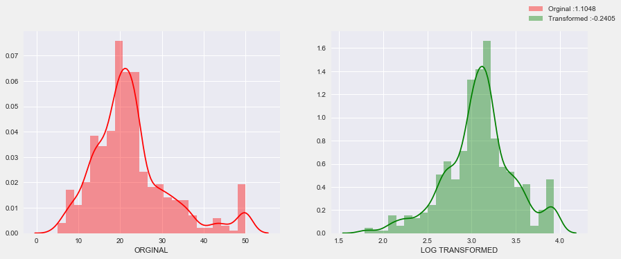
특히 타겟변수가 왜곡된 형태의 분포(skewed)일 경우 예측 성능에 부정적인 영향을 미침
-
로그변환(Log-Transform)
타겟이 right-skewed 상태라면 로그변환을 사용 -> 비대칭 분포형태를 정규분포형태로 변환시켜줌
-
Day 2
Data Wrangling
데이터 랭글링, 분석을 하거나 모델을 만들기 전에 데이터를 사용하기 쉽게 변형하거나 매핑하는 과정
warm upWhen should I use a "groupby" in pandas?
-> when we analyze by category
df.groupby('order_id')['product_id'].count()

= df.groupby('order_id').product_id.count()

df.groupby('order_id')['product_id'].apply(list) # 주문별 구입한 제품들의 product_id를 리스트로

df.groupby('order_id')['prodcut_id'].apply(lambda x: id_Banana in list(x)).value_counts(normalize = True) # 주문에 바나나가 있는 경우 True 리턴

df.groupby('order_id')['banana'].any().value_counts(normalize=True) # 주문(order_id) 중에서 한번이라도 (any()) 바나나 주문이 있으면 Truemerge(on= '') # 칼럼 기준값 설정
merge(left_on = '', right_on ='') # 칼럼명은 다른데 의미는 같은 컬럼일 때 사용Day 3
Feature Importance
warm upBootstrap aggreggation - Bagging
Boosting
AdaBoost
with Decision trees
In a Foreset of Trees made with AdaBoost, the trees are usually just a node and two leaves
stump : A tree with just one node and two leaves -> technically "Week leaner"
1. AdaBoost combines a lot of "week leaners" to make classifications. The week learners are almost always stumps.
2. Some stumps get more say in the classification than others.
3. Each stump is made by taking the previous stump's mistakes into account.Amount of Say : Importance of each stump
Gradient Boosting
When Gradient Boost is ussed to Predict a continuous value, like weight,we say that we are using Gradient Boost for Regression
->Using Gradient Boost for Regression is different from doing Linear Regression
Like AdaBoost, Gradient Boost tree is based on the errors made by the previous tree, but unlike AdaBoost, Gradient Boost tree is usually larger than a stump.
-> Gradient Boost still restricts the size of the tree
Gradient Boost deals with this problem(like low bias and high variance) by using a Learning Rate to scale the contribution from the new tree : Learning Rate is a value between 0 and 1When Gradient Boost is used for Regression, we start with a leaf that is the average value of the variabe we want to Predict.
Then we add a tree based on the Residuals, the difference between the Observed values and the Predicted values and we scale the tree's contribution to the final Prediction with a Learning Rate.
Then we add another tree based on the new Residuals and we keep adding trees based on the errors made by the previous tree.


순열 중요도(Permutation Importances)
특성 중요도 계산 방법
- Feature Importances(Mean decrease impurity, MDI)
sklearn 트리 기반 분류기에서 디폴트로 사용되고 속도는 빠르지만 결과를 주의해서 봐야 함
각각 특성을 모든 트리에 대해 평균불순도감소(mean decrease impurity)를 계산한 값
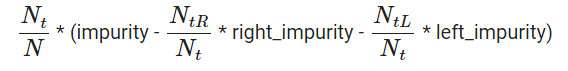
불순도 감소(impurity decrease) 계산
: 전체 관측치 수, : 현재 노드 t에 존재하는 관측치 수
, : 노드 t 왼쪽(L)/오른쪽(R) 자식노드에 존재하는 관측치 수
만약
sample_weight가 주어진다면, , , , 는 가중합Warning: impurity-based feature importances can be misleading for high cardinality features (many unique values). See sklearn.inspection.permutation_importance as an alternative.
-> 범주가 많으면 노드에서 선택될 확률이 높아짐
->전체적인 일반화보단 범주의 종류가 많은 특성들에 그룹에 편향되서 과적합을 일으킴
- Drop-Column Importance
- 매 특성을 drop한 후 fit을 다시 해야 하기 때문에 매우 느리다는 단점
- 특성이 n개 존재할 때 n + 1 번 학습이 필요
- 컬럼 하나씩 제거 -> fit -> score확인 -- n+1 반복
column  = 'opinion_seas_risk'

# opinion_h1n1_risk 없이 fit
pipe = make_pipeline(
    OrdinalEncoder(),
    SimpleImputer(),
    RandomForestClassifier(n_estimators=100, random_state=2, n_jobs=-1)
)
pipe.fit(X_train.drop(columns=column), y_train)
score_without = pipe.score(X_val.drop(columns=column), y_val)
print(f'검증 정확도 ({column} 제외): {score_without}')

# opinion_h1n1_risk 포함 후 다시 학습
pipe = make_pipeline(
    OrdinalEncoder(),
    SimpleImputer(),
    RandomForestClassifier(n_estimators=100, random_state=2, n_jobs=-1)
)
pipe.fit(X_train, y_train)
score_with = pipe.score(X_val, y_val)
print(f'검증 정확도 ({column} 포함): {score_with}')

# opinion_h1n1_risk 포함 전 후 정확도 차이를 계산합니다
print(f'{column}의 Drop-Column 중요도: {score_with - score_without}')- 순열중요도(Permutation Importances, Mean Decrease Accuracy, MDA)
-
기본 특성 중요도와 Drop-column 중요도 중간에 위치하는 특징을 가짐
-
중요도 측정은 관심있는 특성에만 무작위로 노이즈를 주고 예측을 하였을 때 성능 평가지표(정확도, F1, 등)가 얼마나 감소하는지를 측정
-
Drop-column 중요도를 계산하기 위해 재학습을 해야 했다면, 순열중요도는 검증데이터에서 각 특성을 제거하지 않고 특성값에 무작위로 노이즈를 주어 기존 정보를 제거하여 특성이 기존에 하던 역할을 하지 못하게 하고 성능을 측정
- 이때 노이즈를 주는 가장 간단한 방법이 그 특성값들을 샘플들 내에서 섞는 것(shuffle, permutation)
The ELI5 library documentation explains, permutation importance
-
컬럼에 노이즈 주고 -> fit -> score
eli5library
from sklearn.pipeline import Pipeline
# encoder, imputer를 preprocessing으로 묶었습니다. 후에 eli5 permutation 계산에 사용합니다
pipe = Pipeline([
    ('preprocessing', make_pipeline(OrdinalEncoder(), SimpleImputer())),
    ('rf', RandomForestClassifier(n_estimators=100, random_state=2, n_jobs=-1))
])

# pipeline 생성을 확인합니다.
pipe.named_steps

pipe.fit(X_train, y_train)
print('검증 정확도: ', pipe.score(X_val, y_val))

import warnings
warnings.simplefilter(action='ignore', category=FutureWarning)

import eli5
from eli5.sklearn import PermutationImportance

# permuter 정의
permuter = PermutationImportance(
    pipe.named_steps['rf'], # model
    scoring='accuracy', # metric
    n_iter=5, # 다른 random seed를 사용하여 5번 반복
    random_state=2
)

# permuter 계산은 preprocessing 된 X_val을 사용합니다.
X_val_transformed = pipe.named_steps['preprocessing'].transform(X_val)

# 실제로 fit 의미보다는 스코어를 다시 계산하는 작업입니다
permuter.fit(X_val_transformed, y_val);

feature_names = X_val.columns.tolist()
pd.Series(permuter.feature_importances_, feature_names).sort_values() # importance 낮은 순서대로 출력

# 특성별 score 확인
eli5.show_weights(
    permuter,
    top=None, # top n 지정 가능, None 일 경우 모든 특성
    feature_names=feature_names # list 형식으로 넣어야 합니다
)- 중요도가 '-' 인 특성은 제외해도 성능은 거의 영향이 없으며 모델학습 속도는 개선
minimum_importance = 0.001
mask = permuter.feature_importances_ > minimum_importance
features = X_train.columns[mask]
X_train_selected = X_train[features]
X_val_selected = X_val[features]

# pipeline 다시 정의
pipe = Pipeline([
    ('preprocessing', make_pipeline(OrdinalEncoder(), SimpleImputer())),
    ('rf', RandomForestClassifier(n_estimators=100, random_state=2, n_jobs=-1))
], verbose=1)

pipe.fit(X_train_selected, y_train);
Boostiong
분류문제를 풀기 위해서는 트리 앙상블 모델을 많이 사용함
- 트리 앙상블은 랜덤포레스트나 그래디언트 부스팅 모델을 이야기 하며 여러 문제에서 좋은 성능을 보이는 것을 확인
- 트리모델은 non-linear, non-monotonic 관계, 특성간 상호작용이 존재하는 데이터 학습에 적용하기 좋음
- 한 트리를 깊게 학습시키면 과적합을 일으키기 쉽기 때문에. 배깅(Bagging, 랜덤포레스트)이나 부스팅(Boosting) 앙상블 모델을 사용해 과적합을 피함
- 랜덤포레스트의 장점은 하이퍼파라미터에 상대적으로 덜 민감한 것인데, 그래디언트 부스팅의 경우 하이퍼파라미터 셋팅에 따라 랜덤포레스트 보다 더 좋은 예측 성능을 보여줄 수도 있음
부스팅과 배깅의 차이점은?
랜덤포레스트나 그래디언트 부스팅은 모두 트리 앙상블 모델이지만 트리를 만드는 방법에 차이가 있음
-
랜덤포레스트의 경우 각 트리를 독립적으로 만들지만 부스팅은 만들어지는 트리가 이전에 만들어진 트리에 영향을 받는다는 것
-
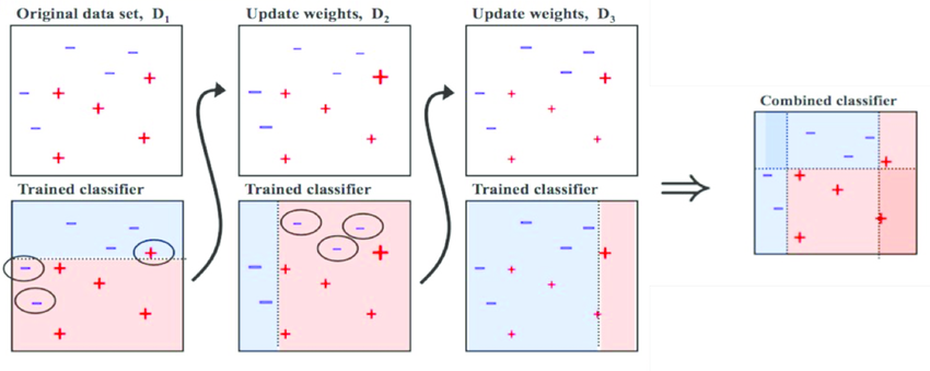
부스팅 알고리즘 중 AdaBoost는 각 트리(약한 학습기들, weak learners)가 만들어질 때 잘못 분류되는 관측치에 가중치를 주고 다음 트리가 만들어질 때 이전에 잘못 분류된 관측치가 더 많이 샘플링되게 하여 그 관측치를 분류하는데 더 초점을 맞춤
AdaBoost의 알고리즘 예시
Step 0. 모든 관측치에 대해 가중치를 동일하게 설정
Step 1. 관측치를 복원추출 하여 약한 학습기 Dn을 학습하고 +, - 분류
Step 2. 잘못 분류된 관측치에 가중치를 부여해 다음 과정에서 샘플링이 잘되도록
Step 3. Step 1~2 과정을 n회 반복(n = 3)
Step 4. 분류기들(D1, D2, D3)을 결합하여 최종 예측을 수행
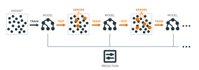
Gradient Boosting
-
회귀와 분류문제에 모두 사용가능
-
그래디언트 부스팅은 AdaBoost와 유사하지만 비용함수(Loss function)을 최적화하는 방법에 있어서 차이가 있음
- 그래디언트 부스팅에서는 샘플의 가중치를 조정하는 대신 잔차(residual)을 학습하도록 하는데 이는 잔차가 더 큰 데이터를 더 학습하도록 만드는 효과가 있음
Python libraries for Gradient Boosting
- scikit-learn Gradient Tree Boosting — 상대적으로 속도가 느릴 수 있습니다.
- Anaconda: already installed
- Google Colab: already installed
- xgboost — 결측값을 수용하며, monotonic constraints를 강제할 수 있습니다.
monotonic constrains 효과, 단조증가해야 하는 특성이 오류로 비단조 증가할때 변수마다 적용 가능
- Anaconda, Mac/Linux:
conda install -c conda-forge xgboost- Windows:
conda install -c anaconda py-xgboost- Google Colab: already installed
- LightGBM — 결측값을 수용하며, monotonic constraints를 강제할 수 있습니다.
- Anaconda:
conda install -c conda-forge lightgbm- Google Colab: already installed
- CatBoost — 결측값을 수용하며, categorical features를 전처리 없이 사용할 수 있습니다.
- Anaconda:
conda install -c conda-forge catboost- Google Colab:
pip install catboost
XGBoost Python API Reference: Scikit-Learn API
from xgboost import XGBClassifier

pipe = make_pipeline(
    OrdinalEncoder(),
    SimpleImputer(strategy='median'),
    XGBClassifier(n_estimators=200
                  , random_state=2
                  , n_jobs=-1
                  , max_depth=7
                  , learning_rate=0.2
                 )
)

pipe.fit(X_train, y_train);
# xgboost 는 랜덤포레스트보다 하이퍼파라미터 셋팅에 민감

from sklearn.metrics import accuracy_score
y_pred = pipe.predict(X_val)
print('검증 정확도: ', accuracy_score(y_val, y_pred))

print(classification_report(y_pred, y_val))
Early Stopping을 사용하여 과적합을 피함
왜 n_estimators 최적화를 위해 GridSearchCV나 반복문 대신 early stopping을?
-
n_iterations가 반복수라 할때, early stopping을 사용하면 우리는n_iterations만큼의 트리를 학습하면 됨 -
하지만 GridSearchCV나 반복문을 사용하면 무려
sum(range(1,n_rounds+1))트리를 학습해야 함 -
거기에
max_depth,learning_rate등등 파라미터 값에 따라 더 돌려야 함
early stopping을 잘 활용하는게 훨씬 효과적
encoder = OrdinalEncoder()
X_train_encoded = encoder.fit_transform(X_train) # 학습데이터
X_val_encoded = encoder.transform(X_val) # 검증데이터

model = XGBClassifier(
    n_estimators=1000,  # <= 1000 트리로 설정했지만, early stopping 에 따라 조절됩니다.
    max_depth=7,        # default=3, high cardinality 특성을 위해 기본보다 높여 보았습니다.
    learning_rate=0.2,
#     scale_pos_weight=ratio, # imbalance 데이터 일 경우 비율을 적용합니다.
    n_jobs=-1
)

eval_set = [(X_train_encoded, y_train),
            (X_val_encoded, y_val)]

model.fit(X_train_encoded, y_train,
          eval_set=eval_set,
          eval_metric='error', # #(wrong cases)/#(all cases)
          early_stopping_rounds=50
         ) # 50 rounds 동안 스코어의 개선이 없으면 멈춤

results = model.evals_result()
train_error = results['validation_0']['error']
val_error = results['validation_1']['error']

epoch = range(1, len(train_error)+1)
plt.plot(epoch, train_error, label='Train')
plt.plot(epoch, val_error, label='Validation')
plt.ylabel('Classification Error')
plt.xlabel('Model Complexity (n_estimators)')
plt.ylim((0.15, 0.25)) # Zoom in
plt.legend();

print('검증 정확도', model.score(X_val_encoded, y_val))
print(classification_report(y_val, model.predict(X_val_encoded)))
하이퍼파라미터 튜닝
Random Forest
- max_depth (높은값에서 감소시키며 튜닝, 너무 깊어지면 과적합)
- n_estimators (적을경우 과소적합, 높을경우 긴 학습시간)
- min_samples_leaf (과적합일경우 높임)
- max_features (줄일 수록 다양한 트리생성, 높이면 같은 특성을 사용하는 트리가 많아져 다양성이 감소)
- class_weight (imbalanced 클래스인 경우 시도)
XGBoost
- learning_rate (높을경우 과적합 위험이 있습니다)
- max_depth (낮은값에서 증가시키며 튜닝, 너무 깊어지면 과적합위험, -1 설정시 제한 없이 분기, 특성이 많을 수록 깊게 설정)
- n_estimators (너무 크게 주면 긴 학습시간, early_stopping_rounds와 같이 사용)
- scale_pos_weight (imbalanced 문제인 경우 적용시도)
baseline model : 기준모델
분류문제: 최빈값
회귀문제 : 평균Learning rate -> overfitting 줄여줌
feature importance에 있던 feature가 permutation에서 사라지면 high cardinality
Day 4
Interpreting ML Model
warm up
Partial dependence plot(PDP) shows the marginal effect one or two features have on the predicted outcome of a machine learning model. PDP can show whether the relationship between the target and a feature is linear, monotonic or more complex.PDP is one of the model-agnostic(모델에 구애받지 않는) way.
PDP는 각 변수들이 서로 상관관계가 없다고 가정하기 때문에 상관성이 너무 높은 변수들이 있다면 PDP적요 전 유의
샘플들의 성질이 매우 다른 경우 PDP는 좋지 못함-> 예측값들을 평균낸 값들로 영향을 보는 것이기 때문에 샘플들의 서로 다른 성질들이 반영되지 못함
Partial Dependence Plots(PDP)
특성들이 타겟에 어떻게 영향을 주는지 쉽게 파악 가능
선형모델은 회귀계수를 이용해 변수와 타겟 관계를 해석 할 수 있지만 트리모델은 불가능
-> PDP 를 사용해 관계 확인
from pdpbox.pdp import pdp_isolate, pdp_plot

feature = 'annual_inc'

isolated = pdp_isolate(
    model=linear,
    dataset=X_val,
    model_features=X_val.columns,
    feature=feature,
    grid_type='percentile', # default='percentile', or 'equal'
    num_grid_points=10 # default=10
)
pdp_plot(isolated, feature_name=feature);
PDP - ICE(Individual Conditional Expectation) curve (: 하나의 관측치에 대해 관심 특성을 변화시킴에 따른 타겟값 변화 곡선) 들의 평균
# PDP곡선을 ICE curves와 함께 그리기

pdp_plot(isolated
         , feature_name=feature
         , plot_lines=True # ICE plots
         , frac_to_plot=0.001 # or 10 (# 10000 val set * 0.001)
         , plot_pts_dist=True)

plt.xlim(20000,150000); #x축 범위 지정
# 한 특성에 대해 PDP를 그릴 경우 얼마나 많은 예측이 필요할까
isolated = pdp_isolate(
model=boosting,
dataset=X_val_encoded,
model_features=X_val.columns,
feature=feature,
# grid point를 크게 주면 겹치는 점이 생겨 Number of unique grid points는 grid point 보다 작을 수 있습니다.
num_grid_points=100, # grid 포인트를 더 줄 수 있습니다. default = 10
)
print('예측수: ',len(X_val) * 100)
# 데이터셋 사이즈에 grid points를 곱한 수 만큼 예측카테고리 특성을 학습할 때 인코딩을 하게 되면 학습 후 PDP를 그릴 때 인코딩된 값이 나옴
-> 해석하는데 어려움
# PDP 카테고리값 매핑 자동으로

feature = 'sex'
for item in encoder.mapping:
    if item['col'] == feature:
        feature_mapping = item['mapping'] # Series

feature_mapping = feature_mapping[feature_mapping.index.dropna()]
category_names = feature_mapping.index.tolist()
category_codes = feature_mapping.values.tolist()

pdp.pdp_plot(pdp_dist, feature)

# xticks labels 설정을 위한 리스트를 직접 넣지 않아도 됩니다
plt.xticks(category_codes, category_names);
2D PDP를 Seaborn Heatmap으로 그리면 카테고리 특성을 매핑 값으로 확인 가능

SHAP
복잡한 머신러닝모델의 예측을 설명하기 위한 매우 유용한 방법
Shapley value를 머신러닝의 특성 기여도(feature attribution) 산정에 활용
사실 특성 갯수가 많아질 수록 Shapley value를 구할 때 필요한 계산량이 기하급수적으로 늘어남
-> SHAP에서는 샘플링을 이용해 근사적으로 값을 구함
- 회귀문제
model = search.best_estimator_
row = X_test.iloc[[1]] # 찾고자 하는 값의 features dataframe

import shap

explainer = shap.TreeExplainer(model)
shap_values = explainer.shap_values(row)

shap.initjs()
shap.force_plot(
    base_value=explainer.expected_value,
    shap_values=shap_values,
    features=row
)
#예측함수 정의

def predict(bedrooms, bathrooms, longitude, latitude):

    # 함수 내에서 예측에 사용될 input을 만듭니다
    df = pd.DataFrame(
        data=[[bedrooms, bathrooms, longitude, latitude]],
        columns=['bedrooms', 'bathrooms', 'long', 'lat']
    )

    # 예측
    pred = model.predict(df)[0]

    # Shap value를 계산합니다
    explainer = shap.TreeExplainer(model)
    shap_values = explainer.shap_values(df)

    # Shap value, 특성이름, 특성값을 가지는 Series를 만듭니다
    feature_names = df.columns
    feature_values = df.values[0]
    shaps = pd.Series(shap_values[0], zip(feature_names, feature_values))

    # 결과를 프린트 합니다.
    result = f'평균가격: ${explainer.expected_value[0]:,.0f} \n'
    result += f'예측가격: ${pred:,.0f}. \n'
    result += shaps.to_string()
    print(result)


    # SHAP Force Plot
    shap.initjs()
    return shap.force_plot(
        base_value=explainer.expected_value,
        shap_values=shap_values,
        features=df
    )

# 각 특성이 어떤 값 범위에서 어떤 영향을 주는지 확인
shap_values = explainer.shap_values(X_test.iloc[:300])
shap.summary_plot(shap_values, X_test.iloc[:300])
- 분류문제
import xgboost
import shap

explainer = shap.TreeExplainer(model)
row_processed = processor.transform(row)
shap_values = explainer.shap_values(row_processed)

shap.initjs()
shap.force_plot(
    base_value=explainer.expected_value,
    shap_values=shap_values,
    features=row,
    link='logit' # SHAP value를 확률로 변환해 표시합니다.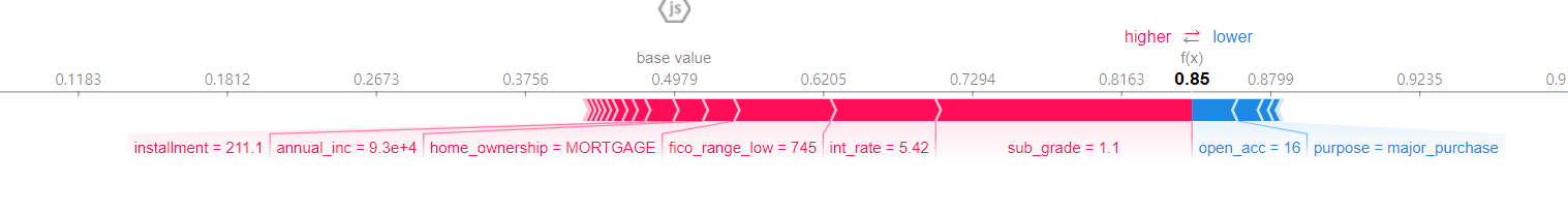
이전 모듈에서 공부한 Feature Importances 와 함께 PDP, SHAP의 특징을 구분해보면
서로 관련이 있는 모든 특성들에 대한 전역적인(Global) 설명
- Feature Importances
- Drop-Column Importances
- Permutaton Importances
타겟과 관련이 있는 개별 특성들에 대한 전역적인 설명
- Partial Dependence plots
개별 관측치에 대한 지역적인(local) 설명
- Shapley Values