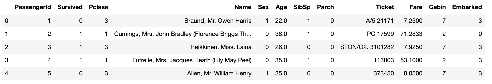
As a review, we will be using train.csv from Kaggle's Titanic dataset to predict the survivors from the disaster.
Input
import numpy as np
import pandas as pd
import matplotlib.pyplot as plt
import seaborn as sns
%matplotlib inline
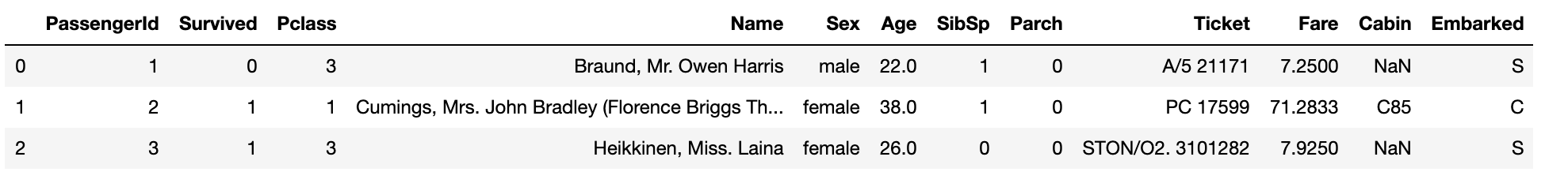
titanic_df = pd.read_csv('titanic_train.csv')
titanic_df.head(3)Output
Previously, we learned it is important to preprocess NULL-type and string-value to train the model. Let us use .info() method to check the column type.
Input
print('Titanic Info ')
print(titanic_df.info()) # Age, Cabin, Embarked have NULL-values
Output
Titanic Info
<class 'pandas.core.frame.DataFrame'>
RangeIndex: 891 entries, 0 to 890
Data columns (total 12 columns):
PassengerId    891 non-null int64
Survived       891 non-null int64
Pclass         891 non-null int64
Name           891 non-null object
Sex            891 non-null object
Age            714 non-null float64
SibSp          891 non-null int64
Parch          891 non-null int64
Ticket         891 non-null object
Fare           891 non-null float64
Cabin          204 non-null object
Embarked       889 non-null object
dtypes: float64(2), int64(5), object(5)
memory usage: 83.7+ KB
None
We can see that columns - Age, Cabin, Embarked have null values. Hence, let us replace NULL using fillna().
Input
# use fillna()
titanic_df['Age'].fillna(titanic_df['Age'].mean(), inplace=True)
titanic_df['Cabin'].fillna('N', inplace=True)
titanic_df['Embarked'].fillna('N', inplace=True)

# check NULL
print('Total Null Values : ', titanic_df.isnull().sum().sum())
Output
Total Null Values : 0Now that we have removed every NULL values, let us encode string-type feature data. First, we will check the distribution of values.
Input
# check distribution of values
print('Sex Distribution: \n', titanic_df['Sex'].value_counts())
print('\nCabin Distribution: \n', titanic_df['Cabin'].value_counts())
print('\nEmbarked Distribution: \n', titanic_df['Embarked'].value_counts())
Output
Sex Distribution:
 male      577
female    314
Name: Sex, dtype: int64

Cabin Distribution:
 N              687
B96 B98          4
C23 C25 C27      4
G6               4
F33              3
              ...
D6               1
C70              1
B73              1
B50              1
C103             1
Name: Cabin, Length: 148, dtype: int64

Embarked Distribution:
 S    644
C    168
Q     77
N      2
Name: Embarked, dtype: int64
We see that columns - Sex and Embarked are evenly distributed, while Cabin shows dispersed feature data values. Assuming the first-alphabet of Cabin represents the level of passenger's cabin, let us extract the first character of each values.
Input
titanic_df['Cabin'] = titanic_df['Cabin'].str[:1]
print(titanic_df['Cabin'].head(3))
Output
0 N
1 C
2 N
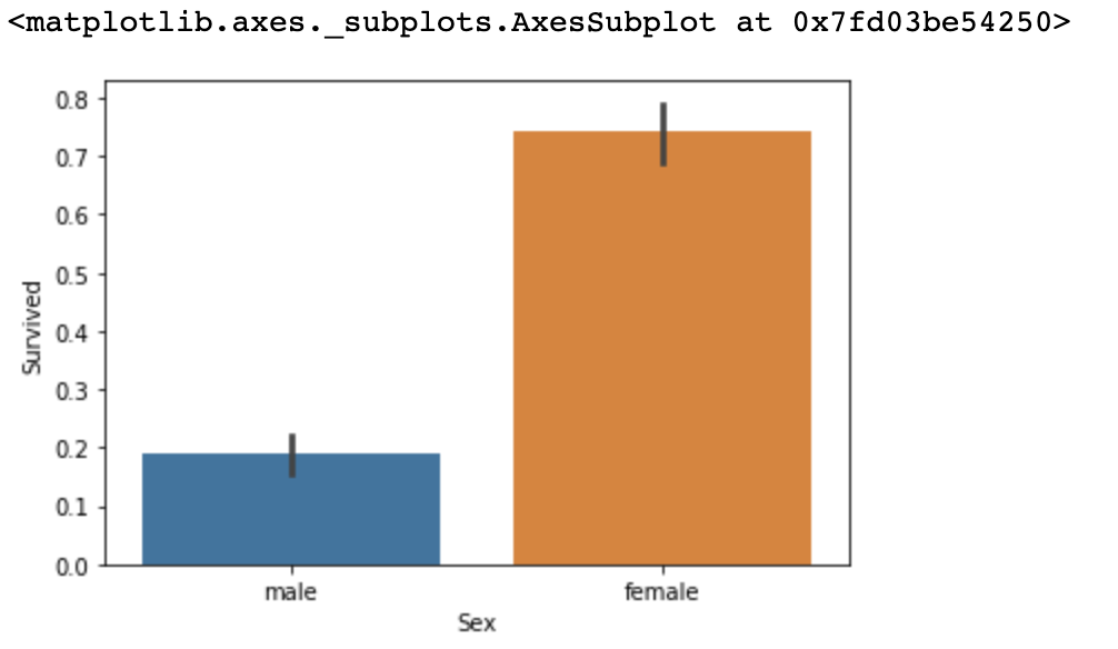
Name: Cabin, dtype: objectBefore we train any model, we will browse through the data. First, let us see what kinds of passengers had higher survival rates. We will compare survival rate based on Sex.
Input
# return pattern of survival
titanic_df.groupby(['Sex', 'Survived'])['Survived'].count()
Output
Sex     Survived
female  0            81
        1           233
male    0           468
        1           109
Input
sns.barplot(x='Sex', y='Survived', data=titanic_df)Output
Now, we will add feature-data Pclass to see if Pclass affected the survival rate within two different sex.
Input
sns.barplot(x='Pclass', y='Survived', hue='Sex', data=titanic_df)Output
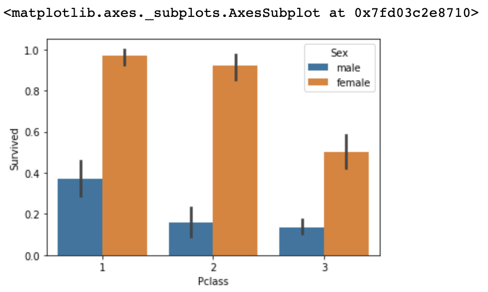
The survival rate of female in Pclass 1 & 2 did not fluctuate by large amounts, but did for Pclass 3.
Now, let us check how Age affected the survival rates. First, let's categorize age into different age-groups.
Input
def get_category(age):
    cat = ''

    if age <= -1: cat = 'Unknown'
    elif age <= 5: cat = 'Baby'
    elif age <= 12: cat = 'Child'
    elif age <= 18: cat = 'Teenager'
    elif age <= 25: cat = 'Student'
    elif age <= 35: cat = 'Young Adult'
    elif age <= 60: cat = 'Adult'
    else: cat = 'Elderly'

    return cat

# adjust graph size
plt.figure(figsize=(10,6))

# display X-values in order
group_names = ['Unknown', 'Baby', 'Child', 'Teenager', 'Student', 'Young Adult', 'Adult', 'Elderly']

titanic_df['Age_cat'] = titanic_df['Age'].apply(lambda x: get_category(x))
sns.barplot(x='Age_cat', y='Survived', hue='Sex', data=titanic_df, order=group_names)

titanic_df.drop('Age_cat', axis=1, inplace=True)
Output
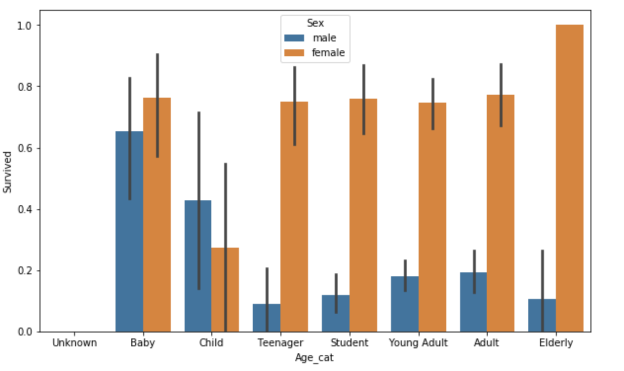
Out of female passengers, Female-elderly had highest survival rate while Female-child had the lowest rate. Female passengers in every age-category had higher survival rates than males.
Based on the analysis so far, we have determined Sex, Age, Pclass are determinant variables to the survival rates.
Now, let us import preprocessing library to encode string-type feature data.
Input
# data encoding
from sklearn import preprocessing

def encode_features(dataDF):
    features = ['Cabin', 'Sex', 'Embarked']

    for feature in features:
        le = preprocessing.LabelEncoder()
        le = le.fit(dataDF[feature])
        dataDF[feature] = le.transform(dataDF[feature])

    return dataDF

titanic_df = encode_features(titanic_df)
titanic_df.head()
Output
We can see that string-type data have all been converted to numerical values.
Now, let us declare multiple functions of pre-processing data to easily convert the dataset.
def fillna(df):
    df['Age'].fillna(df['Age'].mean(), inplace=True)
    df['Cabin'].fillna('N', inplace=True)
    df['Embarked'].fillna('N', inplace=True)
    df['Fare'].fillna(0, inplace=True)

    return df

def drop_features(df):
    df.drop(['Name', 'Ticket', 'PassengerId'], axis=1, inplace=True)

    return df

def format_features(df):
    df['Cabin'] = df['Cabin'].str[:1]
    features = ['Cabin', 'Sex', 'Embarked']

    for feature in features:
        le = preprocessing.LabelEncoder()
        le.fit(df[feature])
        df[feature] = le.transform(df[feature])

    return df

def transform_features(df):
    fillna(df)
    drop_features(df)
    format_features(df)

    return df
Now, reload the data using pd.read_csv() and apply transform_features() that we have called above.
Input
titanic_df = pd.read_csv('titanic_train.csv')
y_titanic_df = titanic_df['Survived']
x_titanic_df = titanic_df.drop('Survived', axis=1)

X_titanic_df = transform_features(x_titanic_df)
Import train_test_split to split the dataset into train & test dataset.
from sklearn.model_selection import train_test_split

X_train, X_test, y_train, y_test = train_test_split(X_titanic_df, y_titanic_df, test_size=0.2, random_state=11)
Let us make three different classifiers to compare the accuracy of each models.
Input
from sklearn.tree import DecisionTreeClassifier
from sklearn.ensemble import RandomForestClassifier
from sklearn.linear_model import LogisticRegression
from sklearn.metrics import accuracy_score

# create classes for classifiers
dt_clf = DecisionTreeClassifier(random_state=11)
rf_clf = RandomForestClassifier(random_state=11)
lr_clf = LogisticRegression()

# Decision Tree
dt_clf.fit(X_train, y_train)
dt_pred = dt_clf.predict(X_test)
print('Decision Tree Accuracy : {0:4f}'.format(accuracy_score(y_test, dt_pred)))

# Random Forest
rf_clf.fit(X_train, y_train)
rf_pred = rf_clf.predict(X_test)
print('Random Forest Accuracy : {0:4f}'.format(accuracy_score(y_test, rf_pred)))

# Logistic Regression
lr_clf.fit(X_train, y_train)
lr_pred = lr_clf.predict(X_test)
print('Logistic Regression Accuracy : {0:4f}'.format(accuracy_score(y_test, lr_pred)))
Output
Decision Tree Accuracy : 0.787709
Random Forest Accuracy : 0.832402
Logistic Regression Accuracy : 0.865922
Logistric Regression returns the highest accuracy of all. However, we can not conclude which algorithm has the best performance since we have not yet finished data optimization.
Now, let us evaluate our classifiers using cross-validation.
Input
from sklearn.model_selection import KFold

def exec_kfold(clf, folds=5):
    # create fold set for the amount of given folds, and list object to contain results
    kfold = KFold(n_splits=folds)
    scores = []

    for iter_count, (train_index, test_index) in enumerate(kfold.split(X_titanic_df)):
        X_train, X_test = X_titanic_df.values[train_index], X_titanic_df.values[test_index]
        y_train, y_test = y_titanic_df.values[train_index], y_titanic_df.values[test_index]

        clf.fit(X_train, y_train)
        predictions = clf.predict(X_test)
        accuracy = accuracy_score(y_test, predictions)
        scores.append(accuracy)

        print('Validation {0} Accuracy: {1:4f}'.format(iter_count, accuracy))

    # calculate average accuracy
    mean_score = np.mean(scores)
    print('Average Accuracy : ', mean_score)

exec_kfold(dt_clf, folds=5)
Output
Validation 0 Accuracy: 0.754190
Validation 1 Accuracy: 0.780899
Validation 2 Accuracy: 0.786517
Validation 3 Accuracy: 0.769663
Validation 4 Accuracy: 0.820225
Average Accuracy :  0.782298662984119
Now let us simply use cross_val_score() to use stratified K-Fold cross validation.
Input
from sklearn.model_selection import cross_val_score

scores = cross_val_score(dt_clf, X_titanic_df, y_titanic_df, cv=5)

for iter_count, accuracy in enumerate(scores):
    print('Validation {0} Accuracy {1}'.format(iter_count, accuracy))

print('\nAverage Accuracy : ', np.mean(scores))
Output
Validation 0 Accuracy 0.7430167597765364
Validation 1 Accuracy 0.776536312849162
Validation 2 Accuracy 0.7808988764044944
Validation 3 Accuracy 0.7752808988764045
Validation 4 Accuracy 0.8418079096045198

Average Accuracy :  0.7835081515022234
However, 78.3% of accuracy-score is yet unsatisfying, hence let us use GridSearch CV to find the best hyper parameter.
We will be creating 5 different fold-sets and evaluate the performance by switching max_depth, min_depth, min_samples_split, and min_samples_leaf.
Input
from sklearn.model_selection import GridSearchCV

parameters = {'max_depth':[2,3,5,10],
             'min_samples_split':[2,3,5], 'min_samples_leaf':[1,5,8]}

grid_dclf = GridSearchCV(dt_clf , param_grid=parameters , scoring='accuracy' , cv=5)
grid_dclf.fit(X_train , y_train)

print('GridSearchCV Best Hyper Parameter :',grid_dclf.best_params_)
print('GridSearchCV Best Accuracy: {0:.4f}'.format(grid_dclf.best_score_))
best_dclf = grid_dclf.best_estimator_

dpredictions = best_dclf.predict(X_test)
accuracy = accuracy_score(y_test , dpredictions)
print('Accuracy of DecisionTreeClassifier In Test-set : {0:.4f}'.format(accuracy))
Ouput
GridSearchCV Best Hyper Parameter : {'max_depth': 3, 'min_samples_leaf': 1, 'min_samples_split': 2}
GridSearchCV Best Accuracy: 0.7992
Accuracy of DecisionTreeClassifier In Test-set : 0.8715
The accuracy increased to 87.15%.