Hi! I'm Jaylnne. 🖐
코드는 아래 Github 레포에! 👇👇👇
0. pytorch lightning 이란?
Pytorch Lightning 이란 Pytorch 에 대한 High-level 인터페이스를 제공하기 위한 라이브러리다. Pytorch 만으로도 충분히 다양한 AI 모델들을 쉽게 생성할 수 있지만 GPU나 TPU, 그리고 16-bit precision, 분산학습 등 더욱 복잡한 조건에서 실험하게 될 경우 코드가 복잡해진다. 코드의 추상화를 통해, 프레임워크를 넘어 하나의 코드 스타일로 자리 잡기 위해 탄생한 프로젝트가 바로 Pytorch Lightning 인 것이다.
Pytorch Lightning 을 사용하면 DataLoader, Model, optimizer, Traning roof 등 딥러닝 모델을 개발할 때 일반적으로 작성하는 코드들을 모두 따로따로 구현해야할 필요가 없어진다. 대신 Lightning Model class 에 이미 구현되어 있는 함수들을 목적에 맞게 적절히 호출하여 사용하기만 하면 된다.
아래는 Pytorch Lightning 의 공식 홈페이지이다. 튜토리얼 영상 등을 통해 Pytorch Lightning 에 대해 친절하게 설명해주고 있으니 들어가서 살펴보면 배울 내용이 많다. 추천! 👍
1. NSMC - 네이버 영화 리뷰 데이터
1-1. NSMC 를 활용하는 이유
주관적인 생각일 뿐이지만, NSMC 가 한국어 NLP 학습셋 중 가장 유명하고 기본적인 데이터셋인 듯하다.
별다른 도메인 지식이 없어도 데이터를 이해하는 데 무리가 없고, 이진분류 태스크 문제라 모델 학습의 난이도도 비교적 낮은 것 같다. 한국어 텍스트 분류 모델의 벤치마킹 데이터로, 각 모델의 성능 비교를 위해서도 많이 사용된다.
이미 사람들에게 많이 알려져 있어서, 데이터에 대한 별도 설명없이 곧바로 모델의 이야기로 넘어갈 수 있다는 점도 많은 사람들이 활용하는 이유이지 않을까 싶다.
참고로 데이터는 아래의 깃헙에서 다운로드 받았다.
1-2. 데이터 설명
Trainset 과 Testset 의 비율은 3:1로 나뉘어져 있다.
- ratings_train.txt : 150K
- ratings_test.txt : 50K
데이터는 아래 3개 컬럼으로 이루어져 있다.
- id: 각 데이터를 식별할 수 있는 key
- document: 리뷰 텍스트
- label: 긍정, 부정 여부
데이터의 예시는 아래와 같다.
$ head ratings_train.txt
id      document        label
9976970 아 더빙.. 진짜 짜증나네요 목소리        0
3819312 흠...포스터보고 초딩영화줄....오버연기조차 가볍지 않구나        1
10265843        너무재밓었다그래서보는것을추천한다      0
9045019 교도소 이야기구먼 ..솔직히 재미는 없다..평점 조정       0
6483659 사이몬페그의 익살스런 연기가 돋보였던 영화!스파이더맨에서 늙어보이기만 했던 커스틴 던스트가 너무나도 이뻐보였다  1
5403919 막 걸음마 뗀 3세부터 초등학교 1학년생인 8살용영화.ㅋㅋㅋ...별반개도 아까움.     0
7797314 원작의 긴장감을 제대로 살려내지못했다.  0
위 예시에서도 보이다시피, txt 확장자 파일이지만 tab 으로 구분되어 있다.
- txt 확장자 파일 👉 tab 구분
1-3. 데이터 정제
working directory 구조
.
├── data
│   ├── ratings_test.txt
│   └── ratings_train.txt
├── Preprocessing.ipynb
├── LICENSE
└── README.md

1 directory, 5 files
위 jaylnne(=나) 의 깃헙에 올려둔 코드로 학습만을 돌려보고자 한다면 데이터를 직접 별도로 다운받지 않아도 된다. DataModule Class 의 prepare_data 함수를 통해, 데이터가 준비되어 있지 않을 경우 자동으로 다운로드 받아지도록 작성해뒀다. 😎
1-3-1. txt 파일 읽어오기
데이터 설명에서 미리 확인했으니, 구분자를 tab 으로 지정하여 pandas dataframe 으로 불러오자. id 컬럼은 사용할 일이 없으니 남겨두지 않고 drop 한다.
import pandas as pd

train = pd.read_csv('data/ratings_train.txt', sep='\t')
test = pd.read_csv('data/ratings_test.txt', sep='\t')

# 필요없는 열은 drop
train.drop(['id'], axis=1, inplace=True)
test.drop(['id'], axis=1, inplace=True)
1-3-2. Null 값 제거하기
# null 개수 확인
print(f'trainset null 개수:\n{train.isnull().sum()}\n')
print(f'testset null 개수:\n{test.isnull().sum()}')
trainset null 개수:
document 5
label 0
dtype: int64
testset null 개수:
document 3
label 0
dtype: int64trainset 에 5개 testset 에 3개 null 값이 존재한다. 제거해주자.
train.dropna(inplace=True)
test.dropna(inplace=True)
1-3-3. 중복 제거하기
document 컬럼을 기준으로 중복 데이터도 삭제해주자.
print(f'중복 제거 전 train length: {len(train)}')
train.drop_duplicates(subset=['document'], inplace=True, ignore_index=True)
print(f'중복 제거 후 train length: {len(train)}\n')
print(f'중복 제거 전 test length: {len(test)}')
test.drop_duplicates(subset=['document'], inplace=True, ignore_index=True)
print(f'중복 제거 후 test length: {len(test)}\n')
중복 제거 전 train length: 149995
중복 제거 후 train length: 146182
중복 제거 전 test length: 49997
중복 제거 후 test length: 491571-3-4. 정규표현식으로 한국어만 남기기
뉴스나 논문 텍스트 데이터와는 달리 댓글 데이터에는 이모티콘과 특수문자도 마구 섞여있다. 우선 정규표현식을 활용해 영어와 한국어 외 특수문자를 없애자.
+) 노이즈 제거 과정에서 발생하는 document 앞뒤 불필요한 공백도 함께 제거한다.
import re
from tqdm import tqdm

def removing_non_korean(df):
    for idx, row in tqdm(df.iterrows(), desc='removing_non_korean', total=len(df)):
        new_doc = re.sub('[^가-힣]', '', row['document']).strip()
        df.loc[idx, 'document'] = new_doc
    return df

train = removing_non_korean(train)
test = removing_non_korean(test)
removing_non_korean: 100%|██████████| 146182/146182 [00:22<00:00, 6366.81it/s]
removing_non_korean: 100%|██████████| 49157/49157 [00:07<00:00, 6368.41it/s]1-3-5. 형태소 분석으로 불필요한 데이터 제거하기
은, 는, 이, 가 등의 조사는 감성분석에 별다른 유의미한 학습 정보를 제공해주지 못할 것이다. mecab 형태소 분석기를 활용하여 조사로 태깅된 토큰들을 제거해주자.
물론 mecab 대신 okt, kkma 처럼 다른 형태소 분석기를 사용해도 된다. 그러나 알려져 있기로 속도면에서는 mecab 을 따라올만 한 분석기가 없다.
이번 nsmc 감성분석 프로젝트에서는 mecab 과 komoran 을 사용해보려고 한다. komoran 은 오탈자를 어느정도 고려해주기 때문에 댓글 데이터에 적절한 것 같다고 생각했기 때문이다.
- mecab
- komoran
a) mecab 형태소 분석기
mecab 은 설치 방법은 아래와 같이 간략하게 정리했다. 나열한 명령어들을 차례대로 터미널에서 실행하면 된다.
(konlpy 공식 문서를 참고했다.)
# mecab 설치
$ sudo apt-get install g++ openjdk-8-jdk python3-dev python3-pip curl
$ pip install konlpy
$ sudo apt-get install curl git
$ bash <(curl -s https://raw.githubusercontent.com/konlpy/konlpy/master/scripts/mecab.sh)
$ pip install mecab-python3
설치가 완료되었다면 mecab 의 품사 태깅표를 확인해보자.
아래와 같이 조사와 어미를 제거해주면 좋을 것 같다.
tags = ['JK', 'JKS', 'JKC', 'JKG', 'JKO', 'JKB', 'JKV', 'JKQ', 'JX', 'JC', 'EP', 'EF', 'EC', 'ETN', 'ETM']from konlpy.tag import Mecab
m = Mecab()
def remove_josa_mecab(df, tags):
for idx, row in tqdm(df.iterrows(), desc='removing josa', total=len(df)):
josa_removed = [x[0] for x in m.pos(row['document']) if x[1] not in tags]
df.loc[idx, 'document'] = ' '.join(josa_removed)
return df
train_mecab = remove_josa_mecab(train, tags)
test_mecab = remove_josa_mecab(test, tags)removing josa: 100%|██████████| 146182/146182 [00:38<00:00, 3791.90it/s]
removing josa: 100%|██████████| 49157/49157 [00:13<00:00, 3700.88it/s]b) komoran 형태소 분석기
위 과정을 통해 konlpy 를 설치했다면 komoran 은 따로 설치할 필요가 없다. konlpy 에서 komoran 클래스도 제공하기 때문이다. komoran 의 품사 태깅표도 mecab 과 같다. 따라서 태그 리스트는 mecab 과 동일하게 하면 된다.
from konlpy.tag import Komoran

k = Komoran()

def remove_josa_komoran(df, tags):
    for idx, row in tqdm(df.iterrows(), desc='removing josa', total=len(df)):
        josa_removed = [x[0] for x in k.pos(row['document']) if x[1] not in tags]
        df.loc[idx, 'document'] = ' '.join(josa_removed)
    return df

train_komoran = remove_josa_komoran(train, tags)
test_komoran = remove_josa_komoran(test, tags)
removing josa: 100%|██████████| 146182/146182 [01:52<00:00, 1302.89it/s]
removing josa: 100%|██████████| 49157/49157 [00:37<00:00, 1323.30it/s]tqdm 을 통해 속도를 비교해보면 확실히 mecab 이 komoran 보다 3~4배 정도 더 빨랐다.
1-3-6. 클래스 분포 확인하기
클래스별 데이터 수가 크게 차이나는, class imbalance 문제가 있는 데이터를 자주 본다. 그런 경우 모델이 특정 클래스에 편향되어 학습될 가능성이 크다. NSMC 도 그렇지 않은지 확인해보자.
import matplotlib.pyplot as plt
plt.style.use('seaborn')

train_mecab_vlcnt = train_mecab['label'].value_counts().reset_index()
train_komoran_vlcnt = train_komoran['label'].value_counts().reset_index()

plt.subplot(1, 2, 1)
plt.title('train_mecab', fontsize=20)
plt.bar(train_mecab_vlcnt['index'], train_mecab_vlcnt['label'], color='skyblue')

plt.subplot(1, 2, 2)
plt.title('train_komoran', fontsize=20)
plt.bar(train_komoran_vlcnt['index'], train_komoran_vlcnt['label'], color='skyblue')

plt.show()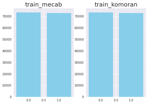
확인 결과, 긍정과 부정 2개 클래스에 데이터가 매우 비슷하게 분포되어 있음을 확인할 수 있다. Class Imbalance 이슈 없음! 🤗
1-3-7. document 길이 분포 확인해보기
koBERT 에 입력으로 들어갈 sequence 의 max length 을 지정하기 위해 document 의 길이 분포를 히스토그램으로 확인해본다.
import numpy as np
import matplotlib.pyplot as plt
plt.style.use('seaborn')

train_mecab_doc_len = [len(x) for x in train_mecab['document']]
train_komoran_doc_len = [len(x) for x in train_komoran['document']]

plt.subplots(constrained_layout=True)

plt.subplot(2, 1, 1)
plt.title('train_mecab', fontsize=20)
plt.hist(train_mecab_doc_len, bins=30)

plt.subplot(2, 1, 2)
plt.title('train_komoran', fontsize=20)
plt.hist(train_komoran_doc_len, bins=30)

plt.show()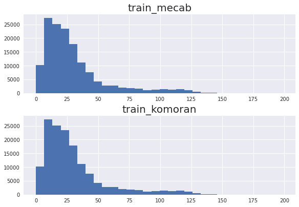
확인해보니 input sequence 의 max length 는 200 정도로 지정해주면 될 듯하다. 전처리가 완료된 데이터를 csv 파일로 저장한다.
train_mecab.to_csv('data/train_mecab.csv', index=False)
test_mecab.to_csv('data/test_mecab.csv', index=False)

train_komoran.to_csv('data/train_komoran.csv', index=False)
test_komoran.to_csv('data/test_komoran.csv', index=False)
2. LightningModule 클래스
이제 전처리가 완료된 데이터를 활용해 파인튜닝하는 과정을 작성해주면 된다. 빈 python 파일 model.py을 하나 생성하고 다음과 같이 LightningModule 클래스 작성으로 시작해보자. (필요한 import 문은 마지막에 한꺼번에 정리할 예정이다.)
2-1. init
class NSMCClassification(pl.LightningModule):

    def __init__(self):
        super(NSMCClassification, self).__init__()

        # load pretrained koBERT
        self.bert = BertModel.from_pretrained('pretrained', output_attentions=True)

        # simple linear layer (긍/부정, 2 classes)
        self.W = nn.Linear(self.bert.config.hidden_size, 2)
self.num_classes = 2-
pytorch lightning 클래스는 항상 pytorch_lightning.LightningModule 을 상속받는다. pytorch 로 모델을 만들 때 nn.Module 을 상속받는 클래스를 만드는 것과 같다고 생각하면 된다.
-
huggingface 로부터 다운받은 koBERT pretained 모델을 불러온다. (모델은 아래의 코드로 'pretrained' 경로에 미리 다운 받아두었다.) NSMC 데이터셋이 한국어이므로, 모델의 종류는 한국어 corpus 로 학습된 kobert 를 택했다.
- jaylnne(=나) 의 깃헙 코드를 활용해 학습만을 돌려보고자 한다면 README.md 를 참고하여
download_pretrained.py를 실행하면 된다.
- jaylnne(=나) 의 깃헙 코드를 활용해 학습만을 돌려보고자 한다면 README.md 를 참고하여
from transformers import BertModel
from kobert_tokenizer import KoBERTTokenizer

model = BertModel.from_pretrained('skt/kobert-base-v1', output_attentions=True)
tokenizer = KoBERTTokenizer.from_pretrained('skt/kobert-base-v1')
model.save_pretrained('pretrained')
tokenizer.save_pretrained('pretrained')- 긍정/부정 2개의 클래스로 텍스트가 분류되어야 하므로, 모델의 output size 를 2차원으로 맞추어주기 위해 linear layer 를 정의해준다.
2-3. forward 함수
이어서 forward 함수의 내용을 작성해보자. 당연한 말이지만, pytorch lightning 에서 정하고 있는 함수명과 동일하게 작성해야한다. 주의!
    def forward(self, input_ids, attention_mask, token_type_ids):

        out = self.bert(
            input_ids=input_ids,
            attention_mask=attention_mask,
            token_type_ids=token_type_ids,
        )

        h_cls = out['last_hidden_state'][:, 0]
        logits = self.W(h_cls)
        attn = out['attentions']

return logits, attn- huggingface 의 BertModel 이 input 을 설정하고, output 에서 logits 값을 파싱해 attention 과 함께 반환하는 forward 함수를 정의한다.
2-4. trainning_step
이제 우리가 정의한 forward 함수가 배치 단위로 어떻게 처리되어야 하는지 training_step 을 정의해보자.
    def training_step(self, batch, batch_nb):
        # batch
        input_ids = batch['input_ids']
        attention_mask = batch['attention_mask']
        token_type_ids = batch['token_type_ids']
        label = batch['label']

        # forward
        y_hat, attn = self.forward(input_ids, attention_mask, token_type_ids)

        # loss
        loss = F.cross_entropy(y_hat, label.long())

        # logs
        tensorboard_logs = {'train_loss': loss}

return {'loss': loss, 'log': tensorboard_logs}-
loss 함수는 Cross Entropy 를 사용한다.
- label 의 type 을 long 으로 변환해주는 것을 잊지 말자.
-
1 배치가 돌 때마다 train_loss 가 떨어지는 걸 확인하며 학습이 잘 이루어지고 있는지 확인하고 싶다. 그래서 train_loss 값을 로깅하도록 했다.
2-5. validation_step 함수
training 과정은 모두 정의해주었으니 validation 단계로 넘어가보자.
    def validation_step(self, batch, batch_nb):
        # batch
        input_ids = batch['input_ids']
        attention_mask = batch['attention_mask']
        token_type_ids = batch['token_type_ids']
        label = batch['label']

        # forward
        y_hat, attn = self.forward(input_ids, attention_mask, token_type_ids)

        # loss
        loss = F.cross_entropy(y_hat, label.long())

        # accuracy
        a, y_hat = torch.max(y_hat, dim=1)
        val_acc = accuracy_score(y_hat.cpu(), label.cpu())
        val_acc = torch.tensor(val_acc)
        self.log('val_acc', val_acc, prog_bar=True)

return {'val_loss': loss, 'val_acc': val_acc}-
1 배치 단위로 실행되는 training_step 을 정의해주었던 것처럼 1 배치 단위로 실행되는 validation_step 을 정의했다. 마찬가지로 batch 를 input 으로 받는다.
-
forward 를 거친 output(=logit) 과 ground_truth(=label) 값으로 loss 를 구하는 과정까지는 같다.
-
그 다음, logit 내 최댓값으로 클래스를 예측하고, 예측 결과와 정답의 비교를 통해 accuracy(val_acc) 를 구한다.
accuracy 를 구하는 과정도 별로 복잡한 건 없다. 다만 torch.max(y_hat, dim=1) 에서 dim=1 부분을 놓치지 않도록 주의하자. logit 의 최댓값 그 자체가 예측 결과가 아니라, logit 내 최댓값의 index 가 예측 label 이어야 하기 때문이다.
# dim=1 설정 여부 차이 확인을 위한 예시
import torch

a = torch.randn(1, 2)

print(f'logit 내 최댓값: {torch.max(a)}')
print(f'logit 내 최댓값의 index: {torch.max(a, dim=1)[1]}')
logit 내 최댓값: -0.4725631773471832
logit 내 최댓값의 index: tensor([0])2-6. validation_end 함수
1 배치가 돌 때마다의 loss 값과 val_acc 를 확인하기 위한 작업을 해주었으니, 이제는 1 epoch 을 돌 때마다의 결과도 확인해볼 수 있도록 하자.
    def validation_end(self, outputs):
        avg_loss = torch.stack([x['val_loss'] for x in outputs]).mean()
        avg_val_acc = torch.stack([x['val_acc'] for x in outputs]).mean()

        tensorboard_logs = {'val_loss': avg_loss,'avg_val_acc':avg_val_acc}
return {'avg_val_loss': avg_loss, 'progress_bar': tensorboard_logs}-
validation_end 의 input 으로 입력될 outputs 는 배치마다 validation_step 이 리턴했던 모든 output 들이다.
-
1 배치마다 계산했던 val_loss 와 val_acc 의 평균을 구해 리턴하고 로그로 출력한다.
2-7. test_step, test_end 함수
validation 단계 작성을 완료했으니 이제는 test 단계로 넘어가면 되겠다. 당연한 말이지만, test 와 관련한 함수들은 모델 학습 과정에서는 사용될 일이 없고, 마지막 epoch 까지 모델 학습이 완료된 이후 우리가 미리 설정해둔 test 데이터셋을 대상으로 실행되게 될 것이다.
    def test_step(self, batch, batch_nb):
        input_ids = batch['input_ids']
        attention_mask = batch['attention_mask']
        token_type_ids = batch['token_type_ids']
        label = batch['label']

        y_hat, attn = self.forward(input_ids, attention_mask, token_type_ids)

        a, y_hat = torch.max(y_hat, dim=1)
        test_acc = accuracy_score(y_hat.cpu(), label.cpu())
        test_acc = torch.tensor(test_acc)

        self.log_dict({'test_acc': test_acc})

        return {'test_acc': test_acc}

    def test_end(self, outputs):
        avg_test_acc = torch.stack([x['test_acc'] for x in outputs]).mean()

        tensorboard_logs = {'avg_test_acc': avg_test_acc}

return {'avg_test_acc': tensorboard_logs}- loss 값을 확인하지 않는다는 차이만 빼면 validation_step, validation_end 과 거의 다르지 않다.
3. Optimizer
optimizer 는 무난하게 Adam 을 활용하기로 하자. optimizer 의 종류는 다양하고 프로젝트의 성격에 따라 적절한 선택을 해주어야하지만, 이번 포스트의 목적은 BERT Classification 파인튜닝을 pytorch lightning 으로 진행해보는 것 그 자체이기 때문에, optimizer 에 대해서는 큰 고민을 하지 않았다.
    def configure_optimizers(self):
        parameters = []
        for p in self.parameters():
            if p.requires_grad:
                parameters.append(p)
            else:
                print(p)

        optimizer = torch.optim.Adam(parameters, lr=2e-05, eps=1e-08)

return optimizer-
self.parameters() 로 interatable 한 parameter 들을 반환한다.
-
그 중 requires_grad 가 Ture 인 것들, 즉 학습이 필요한 parameter 만 parameters 리스트에 모은다. 물론, 현재는 모든 parameter 가 requires_grad 가 True 인 상황일 것이다.
- 🤔 그럼 parameter 의 requires_grad 가 False 인 경우는 언제? ▶ torch.no_grad() 로 gradient 연산을 비활성화 해줄 때가 있다. 당연하게도, validation, test, inference 과정이 여기에 해당할 것이다.
4. Dataset
이 다음 5번에서 작성할 LightningDataModule 클래스의 setup 함수에서 모든 전처리를 진행하는 방법도 있지만, 가독성을 위해 Dataset 클래스를 따로 구성하기로 했다.
class NSMCDataset(Dataset):

    def __init__(self, file_path, max_seq_len):
        self.data = pd.read_csv(file_path)
        self.max_seq_len = max_seq_len
        self.tokenizer = KoBERTTokenizer.from_pretrained('pretrained')

    def __len__(self):
        return len(self.data)

    def __getitem__(self, index):
        data = self.data.iloc[index]

        doc = data['document']
        features = self.tokenizer.encode_plus(str(doc),
                                              add_special_tokens=True,
                                              max_length=self.max_seq_len,
                                              pad_to_max_length='longest',
                                              truncation=True,
                                              return_attention_mask=True,
                                              return_tensors='pt',
                                             )
        input_ids = features['input_ids'].squeeze(0)
        attention_mask = features['attention_mask'].squeeze(0)
        token_type_ids = features['token_type_ids'].squeeze(0)
        label = torch.tensor(data['label'])

        return {
            'input_ids': input_ids,
            'attention_mask': attention_mask,
            'token_type_ids': token_type_ids,
            'label': label
}-
Huggingface tokenizer 의 encode_plus 메소드를 최근 알게 되었는데 굉장히 편리하다. 파라미터를 적절히 설정해주는 것만으로 간편하게 data 를 model 의 input 형태로 만들어줄 수 있다. 자세한 사용법은 아래 공식 문서 페이지를 참조하자.
5. LightningDataModule
간단한 데이터 전처리와 DataLoader 역할을 해줄 LightningDataModule 클래스를 작성해보자.
class NSMCDataModule(pl.LightningDataModule):

    def __init__(self, data_path, mode, valid_size, max_seq_len, batch_size):
        self.data_path = data_path
        self.full_data_path = f'{self.data_path}/train_{mode}.csv'
        self.test_data_path = f'{self.data_path}/test_{mode}.csv'
        self.valid_size = valid_size
        self.max_seq_len = max_seq_len
        self.batch_size = batch_size

    def prepare_data(self):
        # download data
        if not os.path.isfile(f'{self.data_path}/ratings_train.txt'):
            wget.download('https://github.com/e9t/nsmc/raw/master/ratings_train.txt', out=self.data_path)
        if not os.path.isfile(f'{self.data_path}/ratings_test.txt'):
            wget.download('https://github.com/e9t/nsmc/raw/master/ratings_test.txt', out=self.data_path)
        generate_preprocessed(self.data_path)

    def setup(self, stage):
        if stage in (None, 'fit'):
            full = NSMCDataset(self.full_data_path, self.max_seq_len)
            train_size = int(len(full) * (1 - self.valid_size))
            valid_size = len(full) - train_size
            self.train, self.valid = random_split(full, [train_size, valid_size])

        elif stage in (None, 'test'):
            self.test = NSMCDataset(self.test_data_path, self.max_seq_len)

    def train_dataloader(self):
        return DataLoader(self.train, batch_size=self.batch_size, num_workers=5, shuffle=True, pin_memory=True)

    def val_dataloader(self):
        return DataLoader(self.valid, batch_size=self.batch_size, num_workers=5, shuffle=False, pin_memory=True)

    def test_dataloader(self):
return DataLoader(self.test, batch_size=self.batch_size, num_workers=5, shuffle=False, pin_memory=True)-
setup 함수에는 간단한 전처리 로직을 작성해주면 된다. Dataset 클래스 대신 모든 전처리 로직을 setup 함수 아래에 작성해주어도 상관은 없다.
-
주석처리로 비활성화해둔 prepare_data 는 예시처럼 데이터를 다운로드 받거나 클라우드 서버로부터 로드하여 저장하는 로직을 작성하면 된다.
-
왜 setup 과 prepare_data 를 구분해야할까? multi-processing 과 single-processing 의 차이라고 생각하면 된다. setup 은 multi-processing 으로 효율적이고 빠르게 작업이 처리되지만, 데이터 다운로딩까지 multi-processing 으로 이루어진다면 (당연히도) 데이터가 손상되어 버릴 테니까.
-
한 가지 더 주의해야할 점은,
self.data =등과 같이 인스턴스 변수를 prepare_data 에서 설정해주면 안 된다. prepare_data 는 main process 에서만 실행되기 때문이다. prepare_data 에서 인스턴스 변수를 선언한다면 그 데이터는 main process 에 올라간 학습에만 사용될 것이다.
-
6. Trainer
이제 model.py 파일의 내용을 완성했으니 학습을 실행시키는 train.py 파일을 작성해보자.
import torch
import argparse
from pytorch_lightning import Trainer, seed_everything
from pytorch_lightning.callbacks import ModelCheckpoint
from pytorch_lightning.callbacks.early_stopping import EarlyStopping

from model import *


def main():

    parser = argparse.ArgumentParser()
    parser.add_argument('--seed',
                       type=int,
                       default=42)
    parser.add_argument('--data_path',
                        type=str,
                        default='data',
                        help='where to prepare data')
    parser.add_argument('--max_epoch',
                       type=int,
                        default=10,
                       help='maximum number of epochs to train')
    parser.add_argument('--num_gpus',
                       type=int,
                       default=-1,
                       help='number of available gpus')
    parser.add_argument('--mode',
                       type=str,
                       default='clean',
                       choices=['clean', 'only_korean'])
    parser.add_argument('--save_path',
                       type=str,
                       default='checkpoints',
                       help='where to save checkpoint files')
    parser.add_argument('--valid_size',
                       type=float,
                       default=0.1,
                       help='size of validation file')
    parser.add_argument('--max_seq_len',
                       type=int,
                       default=200,
                       help='maximum length of input sequence data')
    parser.add_argument('--batch_size',
                       type=int,
                       default=64,
                       help='batch size')
    args = parser.parse_args()

    seed_everything(args.seed, workers=True)

    dm = NSMCDataModule(
        data_path=args.data_path,
        mode=args.mode,
        valid_size=args.valid_size,
        max_seq_len=args.max_seq_len,
        batch_size=args.batch_size,
    )
    dm.prepare_data()
    dm.setup('fit')

    model = NSMCClassification()

    checkpoint_callback = ModelCheckpoint(
        monitor='val_acc',
        dirpath=args.save_path,
        filename='{epoch:02d}-{val_acc:.3f}',
        verbose=True,
        save_last=False,
        mode='max',
        save_top_k=1,
    )
    early_stopping = EarlyStopping(
        monitor='val_acc',
        mode='max',
    )

    trainer = Trainer(
        max_epochs=args.max_epoch,
        accelerator='gpu',
        strategy="ddp",
        devices=args.num_gpus,
        auto_select_gpus=True,
        callbacks=[checkpoint_callback, early_stopping],
    )
    trainer.fit(model, dm)


if __name__ == '__main__':
main()-
seed_everything 으로 seed 를 고정해 reproductable 한 모델 학습을 진행해보자.
-
pl.callbacks.ModelCheckpoint 로 .ckpt 파일이 저장 방식을 상세히 설정한다. 위 예시에서는 val_acc 가 가장 높은 epoch 의 ckpt 파일을 checkpoint 경로 아래에 저장하게 될 것이다.
-
최대 epoch 수는 10으로 설정해주었지만, Trainer callbacks 옵션에 EarlyStopping 을 추가해주었기 때문에 10 epoch 이 아니더라도 학습이 종료될 수 있다.
-
mecab 과 komoran 두 가지 형태소 분석기를 활용하여 데이터를 생성해두었으니, STEM_ANALYZER 변수를 통해 학습에 활용할 데이터를 선택하도록 했다. ('mecab, 'komoran')생각보다 조사 제거 후 텍스트 길이가 많이 줄어들어서, 조사를 제거하지 않은 데이터도 그대로 사용해보기로 했다. 그 경우에는 STEM_ANALYZER 변수에 'none' 을 넘겨주면 동작하는 방식으로 작성했다.- 실험 결과, 형태소 분석을 거치지 않은 데이터의 학습 결과가 더 좋았으므로,
train.py에 해당 내용을 반영하지는 않기로 했다.
-
병렬 처리 방식은 ddp (= distributed data parallel) 를 택했다. 파이썬의 GIL 의 overhead 를 피하기 위해서다. ddp, dp, GIL 등에 대해 궁금하다면 일전에 작성한 아래 포스트를 읽어보시기를 추천!
<학습 터미널 로그>
$ python train.py

Global seed set to 42
GPU available: True, used: True
TPU available: False, using: 0 TPU cores
IPU available: False, using: 0 IPUs
Global seed set to 42
Global seed set to 42
initializing distributed: GLOBAL_RANK: 1, MEMBER: 2/4
Global seed set to 42
Global seed set to 42
initializing distributed: GLOBAL_RANK: 2, MEMBER: 3/4
Global seed set to 42
Global seed set to 42
initializing distributed: GLOBAL_RANK: 3, MEMBER: 4/4
Global seed set to 42
initializing distributed: GLOBAL_RANK: 0, MEMBER: 1/4
----------------------------------------------------------------------------------------------------
distributed_backend=nccl
All distributed processes registered. Starting with 4 processes
----------------------------------------------------------------------------------------------------

LOCAL_RANK: 0 - CUDA_VISIBLE_DEVICES: [0,1,2,3]
LOCAL_RANK: 3 - CUDA_VISIBLE_DEVICES: [0,1,2,3]
LOCAL_RANK: 1 - CUDA_VISIBLE_DEVICES: [0,1,2,3]
LOCAL_RANK: 2 - CUDA_VISIBLE_DEVICES: [0,1,2,3]

  | Name | Type      | Params
-----------------------------------
0 | bert | BertModel | 92.2 M
1 | W    | Linear    | 1.5 K
-----------------------------------
92.2 M    Trainable params
0         Non-trainable params
92.2 M    Total params
368.754   Total estimated model params size (MB)
Global seed set to 42
Global seed set to 42
Global seed set to 42
Global seed set to 42
Epoch 0: 100%|█████████████████████▉| 1141/1143 [09:35<00:01,  1.98it/s, loss=0.363, v_num=12022-05-03 05:55:21.543166: I tensorflow/stream_executor/platform/default/dso_loader.cc:53] Successfully opened dynamic library libcudart.so.11.0
Epoch 0: 100%|██████████████████████| 1143/1143 [09:37<00:00,  1.98it/s, loss=0.363, v_num=1]Epoch 0, global step 1027: val_acc reached 0.85349 (best 0.85349), saving model to "/data1/jaylnne/nsmc/checkpoints/epoch=00-val_acc=0.853.ckpt" as top 1
Epoch 1: 100%|██████████████████████| 1143/1143 [09:35<00:00,  1.99it/s, loss=0.285, v_num=1]Epoch 1, global step 2055: val_acc reached 0.86573 (best 0.86573), saving model to "/data1/jaylnne/nsmc/checkpoints/epoch=01-val_acc=0.866.ckpt" as top 2
Epoch 2: 100%|███████████████████████| 1143/1143 [09:36<00:00,  1.98it/s, loss=0.23, v_num=1]Epoch 2, global step 3083: val_acc reached 0.86464 (best 0.86573), saving model to "/data1/jaylnne/nsmc/checkpoints/epoch=02-val_acc=0.865.ckpt" as top 3
Epoch 3: 100%|██████████████████████| 1143/1143 [09:35<00:00,  1.99it/s, loss=0.243, v_num=1]Epoch 3, global step 4111: val_acc reached 0.86505 (best 0.86573), saving model to "/data1/jaylnne/nsmc/checkpoints/epoch=03-val_acc=0.865.ckpt" as top 4
Epoch 4: 100%|██████████████████████| 1143/1143 [09:35<00:00,  1.99it/s, loss=0.122, v_num=1]Epoch 4, global step 5139: val_acc reached 0.86436 (best 0.86573), saving model to "/data1/jaylnne/nsmc/checkpoints/epoch=04-val_acc=0.864.ckpt" as top 5
Epoch 4: 100%|██████████████████████| 1143/1143 [09:37<00:00,  1.98it/s, loss=0.122, v_num=1]
학습이 완료되고 나면 CKPT_PATH 변수로 ModelCheckpoint 에 넘겨준 'checkpoints' 경로에 ckpt 파일이 생성된 것을 확인할 수 있다.
.
├── checkpoints
│   └── epoch=01-val_acc=0.866.ckpt
7. test
test.py 파일을 작성해 테스트를 실행해보자. 내용은 train.py 와 거의 유사하다. 체크포인트 경로를 설정해주고, Trainer.fit 대신 Train.test 를 실행해주면 된다. 같은 코드가 반복되는 부분이 많으니 train.py 에서 학습 완료 직후에 곧바로 test 가 실행되게끔 코드를 작성해도 좋다.
import torch
import argparse
from pytorch_lightning import Trainer, seed_everything

from model import *


def main():
    parser = argparse.ArgumentParser()
    parser.add_argument('--seed',
                       type=int,
                       default=42)
    parser.add_argument('--data_path',
                        type=str,
                        default='data',
                        help='where to prepare data')
    parser.add_argument('--num_gpus',
                       type=int,
                       default=-1,
                       help='number of available gpus')
    parser.add_argument('--mode',
                       type=str,
                       default='clean',
                       choices=['clean', 'only_korean'])
    parser.add_argument('--ckpt_path',
                       type=str,
                       help='checkpoint file path')
    parser.add_argument('--valid_size',
                       type=float,
                       default=0.1,
                       help='size of validation file')
    parser.add_argument('--max_seq_len',
                       type=int,
                       default=200,
                       help='maximum length of input sequence data')
    parser.add_argument('--batch_size',
                       type=int,
                       default=32,
                       help='batch size')
    args = parser.parse_args()

    seed_everything(args.seed, workers=True)

    dm = NSMCDataModule(
        data_path=args.data_path,
        mode=args.mode,
        valid_size=args.valid_size,
        max_seq_len=args.max_seq_len,
        batch_size=args.batch_size,
    )
    dm.setup('test')

    model = NSMCClassification()

    trainer = Trainer(
        accelerator='gpu',
        strategy="ddp",
        devices=args.num_gpus,
        auto_select_gpus=True,
    )
    trainer.test(model, dm, ckpt_path=args.ckpt_path)


if __name__ == '__main__':
    main()
전처리 단계별 테스트 결과
아이러니하게도, 전처리를 거치지 않은 데이터의 학습 결과가 가장 좋았다. 😅 빗나간 가정을 했던 듯하다. 뉴스 데이터를 다루어본 경험에 기반한 가정이었는데... 아마도 영화 리뷰 데이터는 뉴스보다 상대적으로 길이가 짧기 때문에, 정보를 최대한 보존하여 학습하는 편이 더 나은 선택이었던 듯하다. 이번 실험에서 mecab 과 komoran 의 차이는 없었다고 봐도 무방하겠다.
| Test Accuracy (%) | Epoch | |
|---|---|---|
| no preprocessing | 89.51% | 5 Epoch |
| none (조사 제거 X) | 88.40% | 3 Epoch |
| mecab | 86.67% | 1 Epoch |
| komoran | 86.67% | 1 Epoch |
8. Next To Do
-
노트북 파일로 작성한 Preprocessing 과정을 파이썬 모듈화할 예정이다.
preprocessing.py생성 완료 ✅
-
하이퍼파라미터를 조금 더 다양하게 조정해가며 실험 결과를 확인해볼 생각이다.
-
텐서보드로 학습 결과를 시각화해볼 예정이다.
-
predict step 과 predict dataloader 를 추가할 예정이다.
-
BentoML 로 도커라이징 & 패키징 후 API 까지 배포할 예정이다.
-
onnx 로 exporting 한 후 inference 속도 변화를 측정해볼 예정이다.
export_to_onnx.py생성 완료 ✅
잘못된 내용이 있으면 댓글로 알려주세요. 감사합니다! 🙇♀️

6개의 댓글

좋은 글 감사합니다.
혹시 Classification class의 forward 구현에서
h_cls = out['last_hidden_state'][:, -1]
이 코드가 어떤 의미인지 알 수 있을까요?
koBERT 공식예제(https://colab.research.google.com/github/SKTBrain/KoBERT/blob/master/scripts/NSMC/naver_review_classifications_pytorch_kobert.ipynb#scrollTo=kLZ9WO0BCkit)
에서는 pooler_output을 Linear 레이어에 input으로 넣는데,
작성해주신 코드에서는 h_cls가 Linear 레이어에 input으로 들어가는 차이가 무엇인지 궁금합니다

안녕하십니까 혹시 긍부정 분류인 Binary 추측이 아닌 네이버댓글 분석결과와 같은 Categorical 추측으로 하는 부분으로 사용하려면 어느 부분을 손봐야하는지 말씀해 주실수 있으신가요?
작성하신 내용과 git 코드 너무 잘 보았습니다.
궁금한게 있는데 학습 모델을 onnx로 생성한후 onnx 모델을 inference 하는 예제도 git에 올려줄 수 있을까요?