Hi! I'm Jaylnne. ✋
이번 포스팅도 [ML] 신용카드 사기 거래 탐지 모델 만들어보기 (2) 과 같이, [ML] 신용카드 사기 거래 탐지 모델 만들어보기 (1) 포스팅에서 개선이 필요했던 내용에 대해 작성한 포스팅입니다.
1. Fix points
(3) 에서 바로잡아보고자 하는 내용은 아래와 같습니다.
- Categorical 변수인
target과 Continuous 변수인predictors의 상관관계를 Pearson Correlation 으로 분석했던 오류
Pandas Dataframe 의 corr 메소드를 활용하면 아주 간단하게 변수들 간의 pearson correlation 을 구할 수 있기 때문에 이러한 실수를 범했던 것 같습니다. 그러나, 곰곰이 짚어보면, 이는 target 인 Class 와 나머지 predictors 변수들간의 상관관계를 분석하기 위한 적절한 방법이 아니었습니다. 왜냐하면 pearson correlation 은 기본적으로 continuous 변수들 간에 선형적인 상관관계가 얼마나 강한지를 보는 분석 기법이기 때문입니다.
2. Why have to fix ?
Pearson Correlation 이 Categorical 변수와의 상관관계 분석에 부적절한 원인을 조금 더 명확히 짚고 넘어가겠습니다. Correlation 이라는 것은 다르게 말해, Standardized Covariance (표준화된 공분산) 입니다. 여기서 covariance, 즉 공분산이라는 건 어떻게 계산되는 값인가요? X 와 Y 라는 두 가지 데이터가 있다고 가정할 때, 두 데이터의 공분산은 X의 편차와 Y의 편차를 곱한 값의 평균 입니다. 아래의 간단한 식을 봐도 매우 명확하죠.
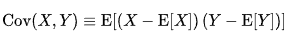
그런데 Categorical 변수는 그 개념이 내포하고 있는 정의상, 이러한 Correlation 계산이 불가합니다. 당장 X 의 편차부터 구하려고 해보아도 말이죠, (X 의 편차를 구하기 위한) X 의 평균을 어떻게 구할 수가 있을까요. 혈액형 A, B, O, AB 형의 평균을 구하라는 말과 같습니다. 혈액형 Categorical 변수의 평균은 BO 라고 말할 수는 없을 테니까요. 😅 이러한 이유로 Pearson Correlation 은 Categorical 변수와 Continuous 변수의 상관관계 분석을 위한 방법으로는 적절하지 않은 것입니다.
2-1. Point biserial Correlation
잠깐! ✋ 여기서 끝내지 않고, 한 가지 질문을 더 던져 보겠습니다.
Categorical 변수가 binary class 이면 조금 달라지는 점이 있을까요?
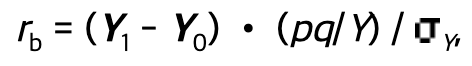
Categorical 변수가 binary class 라는 조건 아래, correlation 을 구할 수 있는 방법이 있습니다. 바로 Pearson Correlation 의 special case 로 볼 수 있는 Point biserial correlation 입니다. 계산식과 조건을 정리하자면 아래와 같습니다.
- One continuous variable
- One naturally binary variable

( 위키피디아 👉 https://en.wikipedia.org/wiki/Point-biserial_correlation_coefficient )
주의해야할 점은, naturally 구분되는 Categorical 변수여야 한다는 것입니다. 예를 들면, 혈액형이나 성별처럼요.
2-2. Biserial Correlation
만약 Categorical 변수가 binary class 이면서, 그 binary class 가 인위적으로 분리된 class 라면 Biserial correlation 를 활용합니다. 인위적으로 분리된 binary class 라고 함은, 시험 합격 또는 불합격을 예로 들 수 있습니다. 실제로는 시험 점수라는 연속된 변수를 특정 점수를 기준으로 두 개의 class 로 인위적으로 분리한 것이죠. 계산식과 조건을 정리하자면 아래와 같습니다.
- One continuous variable
- One artificially divided binary variable
( Ref. 👉 https://www.real-statistics.com/correlation/biserial-correlation/ )
2-3. So, In this case
그렇다면 지난번 작성한 포스팅 - 신용카드 사기 거래 탐지 모델에서 Class (사기 거래 여부) 는 어땠을까요. 분류 모델의 target 이었던 Class 도 정상 거래 또는 사기 거래로 나뉘는 Categorical 변수였습니다. 사기 거래 여부 Class 도 시험 합/불합과 같이 선형적 관계가 내재된 Categorical 변수였을까요, 아니면 혈액형과 같은 경우였을까요?
저는 후자라고 판단했습니다. 따라서 Point Biserial Correlation 으로 feature 들과 target 변수 (=Class) 의 상관관계를 확인해보도록 하겠습니다.
3. 실험 결과
3-1. Calculation & Bar plot
우선 scipy 라이브러리를 활용해 각 feature 들과 Class 간의 point biserial correlation 을 계산하고, 이를 bar plot 으로 그려 높은 상관관계를 띄는 feature 들이 무엇인지 시각적으로 확인해보겠습니다.
# 가장 먼저 필요한 라이브러리들을 미리 임포트해두고...
import time
import numpy as np
import pandas as pd

import scipy.stats as stats

import seaborn as sns
import matplotlib.pyplot as plt

from sklearn.preprocessing import RobustScaler
from sklearn.model_selection import train_test_split, GridSearchCV, cross_validate
from sklearn.linear_model import LogisticRegression
from sklearn.neighbors import KNeighborsClassifier
from sklearn.svm import SVC
from sklearn.tree import DecisionTreeClassifier

# Load data
df = pd.read_csv('data/creditcard.csv')

# Scaling
scaler = RobustScaler()

df['scaled_amount'] = scaler.fit_transform(df['Amount'].values.reshape(-1, 1))
df['scaled_time'] = scaler.fit_transform(df['Time'].values.reshape(-1, 1))

df.drop(['Amount', 'Time'], axis=1, inplace=True)

# Calculate Point Biserial Correlation
features = df.columns.tolist()
features.remove('Class')

corr = {}
for i in features:
    corr[i] = stats.pointbiserialr(df[i], df['Class'])[0]

# Check with Bar plot
x = np.arange(len(corr))
colors = clrs = ['blue' if x < 0 else 'red' for x in corr.values()]
plt.figure(figsize=(30, 10))
plt.bar(x, corr.values(), color=colors)
plt.xticks(x, corr.keys(), rotation=45, fontsize=20)
plt.show()
확인된 Bar plot 은 아래와 같습니다.
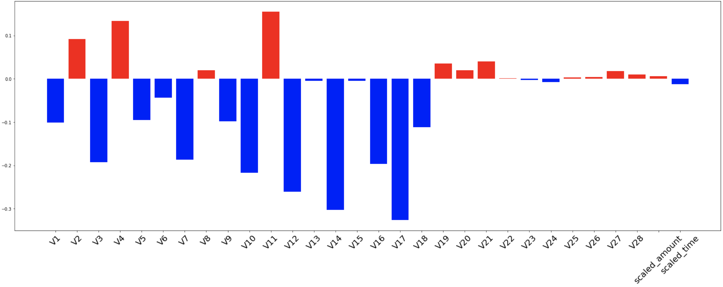
절대값 0.05 이상의 상관관계를 띈 feature 들만 뽑아 정리해보자면 아래와 같습니다.
| 양/음 | feature selection |
|---|---|
| 음의 상관관계 | V1, V3, V5, V7, V9, V10, V12, V14, V16, V17, V18 |
| 양의 상관관계 | V2, V4, V11 |
3-2. Classification
이번에는 point biserial correlation 결과에 기반해 feature selection 을 거친 데이터와, 그렇지 않은 데이터 각각의 classification 결과를 확인해보겠습니다.
✋ 여기서 잠깐! ) 이번 포스팅에서는 기본적으로 correlation 에 기반해, 높은 상관관계를 가진 feature 들만 모델에 활용하는 Filter Method 방식의 feature selection 기법을 적용하고 있습니다. 이 방법론은 발상이 매우 직관적이라 이해가 쉽지만, 사실 기존의 많은 실험들이 이미 해당 방법론만으로는 모델에 적합한 feature 를 정교하게 select 할 수 없음을 보여왔습니다. (오호. Feature Selection 을 주제로 다룬 포스팅을 다음 번에 작성해보면 좋겠네요. 😌 ) 아무튼. 따라서, 이번 포스팅의 실험은 Continuous 변수와 Categorical 변수의 상관관계를 pearson correlation 으로 확인했던 지난 번의 오류를 수정하는 목적에 충실하기 위함임을 이해 부탁드립니다.
# w/ & w/o feature selection
w_df = df[['V1', 'V3', 'V5', 'V7', 'V9', 'V10', 'V12', 'V14', 'V16', 'V17', 'V18', 'V2', 'V4', 'V11', 'Class']]
wo_df = df

def train_and_test(df):
    # Split train and test
    train, test = train_test_split(df, test_size=0.2, shuffle=True, random_state=42, stratify=df['Class'])

    # Under Sampling train dataset
    fraud = train[train['Class']==1].reset_index(drop=True)
    normal = train[train['Class']==0]

    num_of_normal = len(fraud) * 4    # 2:8 비율
    normal = normal.sample(n=num_of_normal, random_state=42, ignore_index=True)
    train = pd.concat([fraud, normal], ignore_index=True)

    # Train Classifier
    X_train = train.drop('Class', axis=1)
    y_train = train['Class']
    X_test = test.drop('Class', axis=1)
    y_test = test['Class']

    model = LogisticRegression(max_iter=10000)
    params = {'penalty':['l2'], 'C':[0.001, 0.01, 0.1, 1, 10, 100, 1000]}
    grid = GridSearchCV(model, params, scoring=['accuracy', 'roc_auc'], refit='roc_auc', return_train_score=True, cv=5)
    grid.fit(X_train, y_train)

    print('< Logistic Regression Results >')
    print(f'Total fit time: {grid.cv_results_["mean_fit_time"].sum()}')
    print(f'The best params: {grid.best_params_}')
    print(f'Test accuracy: {round(grid.score(X_test, y_test) * 100, 2)}%')
    print('\n')

    model = KNeighborsClassifier()
    params = {"n_neighbors": list(range(2,5,1)), 'algorithm': ['auto', 'ball_tree', 'kd_tree', 'brute']}
    grid = GridSearchCV(model, params, scoring=['accuracy', 'roc_auc'], refit='roc_auc', return_train_score=True, cv=5)
    grid.fit(X_train, y_train)

    print('< K-Neighbors Results >')
    print(f'Total fit time: {grid.cv_results_["mean_fit_time"].sum()}')
    print(f'The best params: {grid.best_params_}')
    print(f'Test accuracy: {round(grid.score(X_test, y_test) * 100, 2)}%')
    print('\n')

    model = SVC()
    params = {'C': [0.5, 0.7, 0.9, 1], 'kernel': ['rbf', 'poly', 'sigmoid', 'linear']}
    grid = GridSearchCV(model, params, scoring=['accuracy', 'roc_auc'], refit='roc_auc', return_train_score=True, cv=5)
    grid.fit(X_train, y_train)

    print('< SVC Results >')
    print(f'Total fit time: {grid.cv_results_["mean_fit_time"].sum()}')
    print(f'The best params: {grid.best_params_}')
    print(f'Test accuracy: {round(grid.score(X_test, y_test) * 100, 2)}%')
    print('\n')

    model = DecisionTreeClassifier()
    params = {
        "criterion": ["gini", "entropy"],
        "max_depth": list(range(2,10,1)),
        "min_samples_leaf": list(range(2,10,1))
    }
    grid = GridSearchCV(model, params, scoring=['accuracy', 'roc_auc'], refit='roc_auc', return_train_score=True, cv=5)
    grid.fit(X_train, y_train)

    print('< Decision Tree Results >')
    print(f'Total fit time: {grid.cv_results_["mean_fit_time"].sum()}')
    print(f'The best params: {grid.best_params_}')
    print(f'Test accuracy: {round(grid.score(X_test, y_test) * 100, 2)}%')
    print('\n')
3-2-1. With feature selection
train_and_test(w_df)# output
< Logistic Regression Results >
Total fit time: 0.04124808311462402
The best params: {'C': 0.01, 'penalty': 'l2'}
Test accuracy: 97.71%
< K-Neighbors Results >
Total fit time: 0.01916365623474121
The best params: {'algorithm': 'auto', 'n_neighbors': 4}
Test accuracy: 95.91%
< SVC Results >
Total fit time: 0.19399018287658693
The best params: {'C': 1, 'kernel': 'poly'}
Test accuracy: 97.89%
< Decision Tree Results >
Total fit time: 1.0985085010528564
The best params: {'criterion': 'gini', 'max_depth': 6, 'min_samples_leaf': 9}
Test accuracy: 96.7%3-2-2. Without feature selection
train_and_test(wo_df)# output
< Logistic Regression Results >
Total fit time: 0.17848377227783202
The best params: {'C': 0.01, 'penalty': 'l2'}
Test accuracy: 97.69%
< K-Neighbors Results >
Total fit time: 0.024277877807617185
The best params: {'algorithm': 'auto', 'n_neighbors': 4}
Test accuracy: 95.92%
< SVC Results >
Total fit time: 0.3561769962310791
The best params: {'C': 1, 'kernel': 'rbf'}
Test accuracy: 97.6%
< Decision Tree Results >
Total fit time: 2.4093274116516112
The best params: {'criterion': 'entropy', 'max_depth': 5, 'min_samples_leaf': 9}
Test accuracy: 94.87%3-3-3. Comparision
두 개 실험 결과를 표로 정리해 비교해보자면 아래와 같습니다.
| model | feature selection | test accuracy |
|---|---|---|
| Logistic Regression | O | 97.71% |
| X | 97.69% | |
| KNN | O | 95.91% |
| X | 95.92% | |
| SVC | O | 97.89% |
| X | 97.6% | |
| Decision Tree | O | 96.7% |
| X | 94.87% |
Logistic Regression,SVC,Decision Tree의 경우 with feature selection 가 조금 더 나은 결과를 보였습니다.- without feature selection 조건에서 best model 은
Logistic Regression이었던 것과 달리, feature selection 을 거친 실험에서는SVC가 가장 높은 성능을 보였습니다. - feature selection 전후 가장 많은 성능 차를 보인 것은
Decision Tree였습니다.
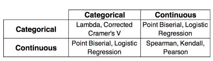
4. 변수의 종류에 따른 correlation
변수의 종류에 따라 어떤 correlation 을 확인하면 좋은지 참고용 표를 아래에 첨부해두겠습니다. 📚