이번 시간에는 저번 시간에 이어 데이터셋을 이용하여 SVM을 활용해 보도록 하겠습니다.
데이터셋 불러오기
input
from sklearn.datasets import make_blobs
X,y=make_blobs(n_samples=100, centers=2, cluster_std=0.5, random_state=0)
blobs라는 데이터 셋을 모듈을 사용하여 불러옵니다.
데이터 시각화
input
import matplotlib.pyplot as plt
plt.scatter(X[y==0, 0], X[y==0, 1], marker='o', label='class 0')
plt.scatter(X[y==1, 0], X[y==1, 1], marker='x', label='class 1')
plt.xlabel('x1')
plt.ylabel('x2')
plt.legend()
plt.show()
output

불러온 데이터의 분포를 확인하기 위해서 데이터를 시각화해 줍니다.
데이터 분류 및 학습
input
from sklearn.model_selection import train_test_split
from sklearn.svm import SVC
X_train, X_test, y_train, y_test=train_test_split(X,y,test_size=0.2, stratify=y, random_state=0)
model=SVC(kernel='linear').fit(X_train,y_train)
train과 test(연습과 검증)데이터로 분류하고 지난 시간에 배운 SVC함수로 데이터를 학습해 줍니다.
input
import numpy as np
def plot_svc(model, ax=None):
    if ax==None:
        ax=plt.gca() #새로운 그래픽 객체 생성
    xlim=ax.get_xlim()
    ylim=ax.get_ylim()
    x=np.linspace(xlim[0], xlim[1], 30)
    y=np.linspace(ylim[0], ylim[1], 30)
    Y, X=np.meshgrid(y,x) #정방행렬
    xy=np.vstack([X.ravel(), Y.ravel()]).T  #행렬 전치
    P=model.decision_function(xy).reshape(X.shape) #판별함수에 입력
    #등고선 그래프
    ax.contour(X,Y,P,levels=[-1,0,1],linestyles=['--','-','--'])
    ax.scatter(model.support_vectors_[:,0], model.support_vectors_[:,1],s=200)
    ax.set_xlim(xlim)
    ax.set_ylim(ylim)
plt.scatter(X_train[:,0], X_train[:,1], c=y_train, s=50, cmap='winter')
X_new=[1.5, 2.5]
plt.plot(X_new[0], X_new[1], 'x', color='red', markersize=20)
plot_svc(model)
output
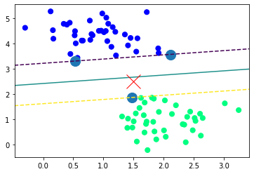
데이터를 시각화 및 최적의 초평면과 최대 마진, 새로운 데이터 입력시 예측을 하기위한 프로그래밍을 해줍니다.
최적화(파이프라인)
input
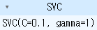
from sklearn.model_selection import GridSearchCV
params={'C': [0.1, 1, 10, 100], 'gamma': [1, 0.1, 0.01, 0.001, 0.00001, 10]}
grid=GridSearchCV(SVC(), params)
grid.fit(X_train, y_train)
print(grid.best_params_)
print(grid.best_estimator_)
output
{'C': 0.1, 'gamma': 1}
SVC(C=0.1, gamma=1)
파이프라인을 이용하여 최적화를 시켜줍니다. C와 Gamma에 대해서는 다음시간에 좀 더 자세히 다루어 보도록하겠습니다.
정확도 출력
input
model=grid.best_estimator_
model
print(model.score(X_train,y_train))
print(model.score(X_test,y_test))
output
1.0
1.0
최적화한 데이터로 모델을 학습 시켜 정확도로 출력하니 100%가 되었습니다.
이번에는 사진을 이용한 데이터를 학습시켜 보도록 하겠습니다.
데이터셋 불러오기
input
from sklearn.datasets import fetch_olivetti_faces
faces=fetch_olivetti_faces()
print(len(faces.data)) # 400개의 이미지
print(set(faces.target)) # 40 class
output
downloading Olivetti faces from https://ndownloader.figshare.com/files/5976027 to C:\Users\user\scikit_learn_data
400
{0, 1, 2, 3, 4, 5, 6, 7, 8, 9, 10, 11, 12, 13, 14, 15, 16, 17, 18, 19, 20, 21, 22, 23, 24, 25, 26, 27, 28, 29, 30, 31, 32, 33, 34, 35, 36, 37, 38, 39}
데이터 시각화
input
import matplotlib.pyplot as plt
import numpy as np
N=2
M=5
#np.random.seed(0)
fig=plt.figure(figsize=(9,5))
klist=np.random.choice(range(len(faces.data)),N*M) #10개 선택
for i in range(N):
    for j in range(M):
        k=klist[i*M+j]
        ax=fig.add_subplot(N,M,i*M+j+1)
        ax.imshow(faces.images[k], cmap=plt.cm.gray) #이미지 출력
        ax.xaxis.set_ticks([]) #x축 눈금 제거
        ax.yaxis.set_ticks([]) #y축 눈금 제거
        plt.title(faces.target[k])
plt.tight_layout()
plt.show()
output
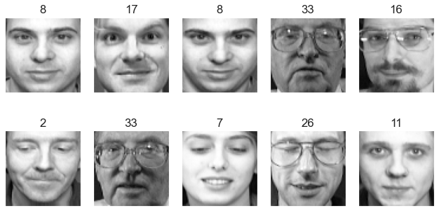
pyplot함수를 이용하여 데이터를 10개씩 시각화하여 출력하는 코드입니다.
데이터분류 및 학습
input
from sklearn.model_selection import train_test_split
from sklearn.svm import SVC
X_train,X_test,y_train,y_test=train_test_split(faces.data, faces.target, stratify=faces.target, test_size=0.2, random_state=0)
svc=SVC().fit(X_train,y_train)
연습 검증으로 데이터를 분류하고 학습시켜줍니다.
데이터 시각화 및 검증
input
N = 2
M = 5
np.random.seed(4)
fig = plt.figure(figsize=(9, 5))
klist = np.random.choice(range(len(y_test)), N * M)
for i in range(N):
    for j in range(M):
        k = klist[i * M + j]
        ax = fig.add_subplot(N, M, i * M + j + 1)
        # 이미지 출력을 위해 2차원 데이터로 변환
        ax.imshow(X_test[k:(k + 1), :].reshape(64, 64), cmap=plt.cm.gray)
        ax.xaxis.set_ticks([])
        ax.yaxis.set_ticks([])
        pred=svc.predict(X_test[k:(k + 1), :])[0]
        plt.title(f"{y_test[k]} => {pred}")

plt.tight_layout()
plt.show()
output
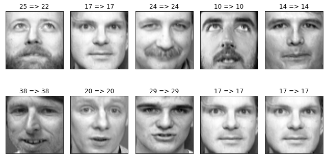
학습시킨 모델의 정확도를 알기위한 코드입니다. N 세로 M 가로 2줄 5개씩 총 10개의 사진을 출력을 시키며 데이터를 각각 데이터를 예측하기 위해 2차원으로 변환 시킨 후 {실제값} => {예측값}을 출력하게 했습니다. 1번 데이터 값의 예측이 틀렸음을 알 수 있습니다.
정확도출력
input
print(svc.score(X_train,y_train))
print(svc.score(X_test,y_test))
output
1.0
0.95
0.5%의 과적합이 일어 났습니다.
혼동행렬을 이용한 평가지표 확인
input
from sklearn.metrics import confusion_matrix, classification_report
import pandas as pd
import seaborn as sns

pred=svc.predict(X_test)
cm=confusion_matrix(y_test, pred)
df_cm=pd.DataFrame(cm, index=range(0,40), columns=range(0,40))
sns.set(font_scale=1.4)
plt.figure(figsize=(15,10))
sns.heatmap(df_cm, annot=True)
plt.show()
output

학습시킨 모델의 학습력에 따른 정확도 향상을 확인 할 수 있습니다.
평가지표 확인 2
input
print(classification_report(y_test, pred))output

classification_report함수를 이용하여 시각화한 데이터를 문서화하여 필요한 데이터를 필요한 부분을 따로 출력할 수 있습니다.
이번시간에는 여러가지 데이터셋을 이용하여 SVM으로 학습시키는 방법을 배워보았습니다. 다음 시간에는 이번 시간에 나온 C, Gamma에 대해 자세히 다루어 보도록하겠습니다.
😁 power through to the end 😁