텐서플로우 공식문서
텐서플로우 API

1. 텐서플로우 Tensorflow란?

텐서플로 또는 텐서플로우는 다양한 작업에대해 데이터 흐름 프로그래밍을 위한 오픈소스 소프트웨어 라이브러리이다. 심볼릭 수학 라이브러리이자, 인공 신경망같은 기계 학습 응용프로그램 및 딥러닝에도 사용된다.

TensorFlow와 Keras는 ML 모델을 개발하고 학습시키는 데 도움이 되는 핵심 오픈소스 라이브러리입니다.

텐서플로우와 케라스

TensorFlow와 Keras는 모두 2015년에 릴리즈 되었습니다 (Keras는 2015년 3월, TensorFlow는 2015년 11월). 이는 딥러닝 세계의 관점에서 볼 때, 꽤 오랜시간이라고 볼 수 있습니다.

Keras는 사용자가 TensorFlow를 좀 더 쉽고 편하게 사용할 수 있게 해주는 high level API를 제공합니다.

TensorFlow 2.x에서는 Keras를 딥러닝의 공식 API로 채택하였고, Keras는 TensorFlow 내의 하나의 framwork으로 개발되고 있습니다.

2. TensorFlow / Keras Tutorial

• 코랩으로 작성하고 깃허브에 업로드 하였음
  https://github.com/Junga15/python-library/blob/main/Ch03탠서플로우케라스이론및실습_TensorFlow_Keras_Tutorial.ipynb

TensorFlow / Keras import

import tensorflow as tf
from tensorflow import keras

print(tf.__version__)
print(keras.__version__)
2.8.2
2.8.0

TensorFlow / Keras 맛보기 : mnist 데이터

import numpy as np
import matplotlib.pyplot as plt

# MNIST dataset download
mnist = keras.datasets.mnist #사람이 손으로 쓴 손글씨 숫자

(x_train, y_train), (x_test, y_test) = mnist.load_data()
x_train, x_test = x_train / 255.0, x_test / 255.0

mnist = keras.datasets.mnist

(x_train, y_train), (x_test, y_test) = mnist.load_data()
x_train, x_test = x_train /255.0, x_test / 255.0

# Model 생성, compile
model = tf.keras.models.Sequential([
  tf.keras.layers.Flatten(input_shape=(28, 28)),
  tf.keras.layers.Dense(128, activation='relu'),
  tf.keras.layers.Dropout(0.2),
  tf.keras.layers.Dense(10, activation='softmax')
])

model.compile(optimizer='adam',
              loss='sparse_categorical_crossentropy',
              metrics=['accuracy'])

# Training / Evaluation
model.fit(x_train, y_train, epochs=10)

model.evaluate(x_test,  y_test)

Epoch 1/10
1875/1875 [==============================] - 4s 2ms/step - loss: 0.0406 - accuracy: 0.9861
Epoch 2/10
1875/1875 [==============================] - 4s 2ms/step - loss: 0.0377 - accuracy: 0.9872
....
Epoch 9/10
1875/1875 [==============================] - 4s 2ms/step - loss: 0.0266 - accuracy: 0.9908
Epoch 10/10
1875/1875 [==============================] - 6s 3ms/step - loss: 0.0247 - accuracy: 0.9915
313/313 [==============================] - 1s 3ms/step - loss: 0.0874 - accuracy: 0.9793
[0.08744390308856964, 0.9793000221252441]

# 데이터 탐색
idx = np.random.randint(len(x_train))
image = x_train[idx]

plt.imshow(image, cmap='gray')
#plt.title(x_train[idx])
plt.title(y_train[idx])
plt.show()

내가 쓴 손글씨로 Test 해봅시다.
Colab을 쓰는 경우에는 아래 cell을 실행하면 파일을 업로드할 수 있습니다.
그림판과 같은 도구를 이용하여 손으로 숫자를 쓴 다음 파일로 저장하고 업로드 합니다.
이 때 파일명은 image.png로 합니다.

import os
from PIL import Image
from google.colab import files #구글 코랩으로부터 files 패키지를 임포트함

uploaded = files.upload() #files.upload() 함수를 통해 파일 업로드 실행

for fn in uploaded.keys(): #업로드된 파일 정보를 출력하는 코드
  print('User uploaded file "{name}" with length {length} bytes'.format(
      name=fn, length=len(uploaded[fn]))) #name = fn = uploaded.keys()의 예: image.png, 삼.png, length=len(uploaded[fn])의 예: 907 bytes (1KB )

# image file의 경로 설정
cur_dir = os.getcwd() #/content
img_path = os.path.join(cur_dir, 'image.png')
# image file 읽기
cur_img = Image.open(img_path)
# 28x28로 resize
cur_img = cur_img.resize((28, 28))
image = np.asarray(cur_img) # 이미지를 넘파이 어레이로 바꿈

# color image일 경우 RGB 평균값으로 gray scale로 변경
try:
  image = np.mean(image, axis=2) #RGB를 평균내서 흑백으로 바꿔버림★, axis=2는 행평균
                                #※np.mean, axis=2 : 행평균
                                # https://s-engineer.tistory.com/255
                                # axis = 0 원소별 평균, axis = 1은 열평균

except:
  pass
image = np.abs(255-image) #색 반전: upload한 image는 흰 배경에 검은 글씨로 되어 있으므로, MNIST data와 같이 검은 배경에 흰 글씨로 변경
# MNIST와 동일하게 data preprocessing(255로 나눠줌)
image = image.astype(np.float32)/255. #파이썬 astype함수: 데이터타입 변경함수, 255로 나눠서 픽셀값이 0~1사이에 들어올 수 있도록 해줌
# 화면에 출력하여 확인
plt.imshow(image, cmap='gray')
plt.show()

# shape을 변경하여 학습된 model에 넣고 결과 확인
image = np.reshape(image, (1, 28, 28)) #(1, 28, 28) : 1장의 이미지가 들어갈 것이다.(배치사이즈), 그림 크기 28 *28 픽셀
                                       # reshape을 통해 차원을 하나 더 늘려줌
print(model.predict(image))

print("Model이 예측한 값은 {} 입니다.".format(np.argmax(model.predict(image), -1))) #np.argmax : 최대값 위치반환, axis=-1은 1번축(가로축,행방향)에서 제일 큰 놈 위치 반환 https://jimmy-ai.tistory.com/72

# [[2.0712188e-14 5.9028615e-11 7.3312776e-08 9.9999881e-01 1.4067702e-14
#   3.2937263e-07 6.1719135e-17 1.8426191e-07 6.1457428e-07 1.7880680e-11]]
# :순서대로, 0일 확률, 1일 확률, 2일 확률, 3일 확률, 4일 확률
#            5일 확률, 6일 확률, 7일 확률, 8일 확률, 9일확률
# Model이 예측한 값은 [3] 입니다.
#=> 모델훈련 결과가 정확도가 97%나오는 모델이어서 잘 예측함

1. TensorFlow / Keras 기본 사용 문법

1. Tensor

Tensor는 multi-dimensional array를 나타내는 말로, TensorFlow의 기본 data type입니다

• 1. tf.constant : 텐서 생성

# 텐서 생성 : tf.constant
hello = tf.constant([3,3], dtype=tf.float32) # 넘파이와 비슷함
print(hello) #tf.Tensor([3. 3.], shape=(2,), dtype=float32) : 텐서같은 경우에는 shape과 데이터타입 모두 나옴

tf.Tensor([3. 3.], shape=(2,), dtype=float32)

hello = tf.constant('helloworld')
print(hello) #tf.Tensor(b'helloworld', shape=(), dtype=string) #shape은 없고, 데이터타입은 문자열

tf.Tensor(b'helloworld', shape=(), dtype=string)

# 상수형 tensor는 아래와 같이 만들 수 있습니다
# 출력해보면 tensor의 값과 함께, shape과 내부의 data type을 함께 볼 수 있습니다
x = tf.constant([[1.0, 2.0],
                 [3.0, 4.0]])
print(x)
print(type(x)) #<class 'tensorflow.python.framework.ops.EagerTensor'> EagerTensor: 결과가 바로바로 나오게 해주는 것, 1점대에서는 그냥 tensor였음

tf.Tensor(
[[1. 2.]
 [3. 4.]], shape=(2, 2), dtype=float32)
<class 'tensorflow.python.framework.ops.EagerTensor'>

• 2. tf.convert_to_tensor : numpy array와 파이썬 리스트를 텐서tensor로 변경

# 아래와 같이 numpy ndarray나 python의 list도 tensor로 바꿀 수 있습니다
x_np = np.array([[1.0, 2.0],
                [3.0, 4.0]])
x_list = [[1.0, 2.0], 
         [3.0, 4.0]]

print(type(x_np))
print(type(x_list))

<class 'numpy.ndarray'>
<class 'list'>

x_np = tf.convert_to_tensor(x_np)
x_list = tf.convert_to_tensor(x_list)

print(type(x_np))
print(type(x_list))

<class 'tensorflow.python.framework.ops.EagerTensor'>
<class 'tensorflow.python.framework.ops.EagerTensor'>

# 반대로 tensor를 다음과 같이 numpy ndarray로 바꿀 수도 있습니다
x.numpy()

array([[1., 2.],
       [3., 4.]], dtype=float32)
       
print(type(x.numpy()))   
<class 'numpy.ndarray'>
       
a = tf.ones((2,3))
b = tf.zeros((2,3))
c = tf.fill((2,2), 2) #np.full
print(a)
print(b)
print(c)

tf.Tensor(
[[1. 1. 1.]
 [1. 1. 1.]], shape=(2, 3), dtype=float32)
tf.Tensor(
[[0. 0. 0.]
 [0. 0. 0.]], shape=(2, 3), dtype=float32)
tf.Tensor(
[[2 2]
 [2 2]], shape=(2, 2), dtype=int32)
 
d = tf.zeros_like(c) #모양만 가져오는 것이 아닌 데이터타입도 가져옴, dtype=int32
e = tf.ones_like(c) 
print(d)
print(e)

tf.Tensor(
[[0 0]
 [0 0]], shape=(2, 2), dtype=int32)
tf.Tensor(
[[1 1]
 [1 1]], shape=(2, 2), dtype=int32)

f = tf.eye(3) #항등행렬
print(f)
tf.Tensor(
[[1. 0. 0.]
 [0. 1. 0.]
 [0. 0. 1.]], shape=(3, 3), dtype=float32)
 
g  = tf.range(10)
print(g)
tf.Tensor([0 1 2 3 4 5 6 7 8 9], shape=(10,), dtype=int32)

h = tf.random.uniform((2,2)) # np.rand 0~1 균등분포 중 뽑음 => 최대값, 최소값 지정 가능하나 기본은 0~1사이
i = tf.random.normal((2,2))  # np.randn 표준정규분포(normal distribution: 평균0, 표준편차1)에서 뽑음
print(h)
print(i)

tf.Tensor(
[[0.6857052  0.47401726]
 [0.68458676 0.41493607]], shape=(2, 2), dtype=float32)
tf.Tensor(
[[-1.8853602   1.4278084 ]
 [ 2.4465408  -0.49401993]], shape=(2, 2), dtype=float32)

• 3. Tensor의 속성

tensor = tf.random.normal((3,4))

print(f"Shape of tensor: {tensor.shape}")
print(f"Datatype of tensor: {tensor.dtype}")

Shape of tensor: (3, 4)
Datatype of tensor: <dtype: 'float32'>

# 속성 변경 : tf.cast
tensor = tf.reshape(tensor, (4, 3))
tensor = tf.cast(tensor, tf.int32) 

print(f"Shape of tensor: {tensor.shape}")
print(f"Datatype of tensor: {tensor.dtype}")

Shape of tensor: (4, 3)
Datatype of tensor: <dtype: 'int32'>

2. Variable

Variable은 변할 수 있는 상태를 저장하는데 사용되는 특별한 텐서입니다.
딥러닝에서는 학습해야하는 가중치(weight, bias)들을 variable로 생성합니다.

# tensor의 값 변경 - 변경 불가능
tensor = tf.ones((3,4))
print(tensor)

tensor[0,0] = 2. #에러뜸, 파이썬의 튜플처럼 텐서는 한번 값을 생성하면 값을 변경할 수 없다. 
                 #TypeError: 'tensorflow.python.framework.ops.EagerTensor' object does not support item assignment
                 #텐서의 값을 변경하기 위해 tf.Variable을 사용함 ex>weight값들은 처음에 random한 값을 채운다음에 학습이 진행되면서 웨이트값 업데이트 되어야 하기 때문에 그때 사용
                 
                 
tf.Tensor(
[[1. 1. 1. 1.]
 [1. 1. 1. 1.]
 [1. 1. 1. 1.]], shape=(3, 4), dtype=float32)
---------------------------------------------------------------------------
TypeError                                 Traceback (most recent call last)
<ipython-input-47-09e82e60b3e3> in <module>()
      3 print(tensor)
      4 
----> 5 tensor[0,0] = 2.

TypeError: 'tensorflow.python.framework.ops.EagerTensor' object does not support item assignment                 

• 1. tf.Variable

# variable 만들기, 값 변경
variable = tf.Variable(tensor) #tensor: 이자리에 들어가는 것이 weight 초기값
print(variable)

variable[0,0].assign(2) #0컴마0자리 2로 변경됨
print(variable)

<tf.Variable 'Variable:0' shape=(3, 4) dtype=float32, numpy=
array([[1., 1., 1., 1.],
       [1., 1., 1., 1.],
       [1., 1., 1., 1.]], dtype=float32)>
<tf.Variable 'Variable:0' shape=(3, 4) dtype=float32, numpy=
array([[2., 1., 1., 1.],
       [1., 1., 1., 1.],
       [1., 1., 1., 1.]], dtype=float32)>

# 초기값을 사용해서 Variable을 생성할 수 있습니다
initial_value = tf.random.normal(shape=(2, 2)) 
weight = tf.Variable(initial_value)
print(weight)
<tf.Variable 'Variable:0' shape=(2, 2) dtype=float32, numpy=
array([[-1.1036984 ,  0.18638368],
       [ 1.0083843 ,  0.2881591 ]], dtype=float32)>
       
# 아래와 같이 variable을 초기화해주는 initializer들을 사용할 수도 있습니다
weight = tf.Variable(tf.random_normal_initializer(stddev=1.)(shape=(2,2))) #random_normal_initializer(stddev=1.평균,표준편차 변경가능)(shape=(2,2)
print(weight)
<tf.Variable 'Variable:0' shape=(2, 2) dtype=float32, numpy=
array([[-1.1520137 ,  0.23932126],
       [ 0.04164846,  0.99494994]], dtype=float32)>
       
# variable은 `.assign(value)`, `.assign_add(increment)`, 또는 `.assign_sub(decrement)`
# 와 같은 메소드를 사용해서 Variable의 값을 갱신합니다:'''

new_value = tf.random.normal(shape=(2,2))
print(new_value)
weight.assign(new_value) #assign을 통한 Variable 값(weight) 갱신
print(weight) #뉴밸류값이 웨이트값이 됨       

added_value = tf.ones(shape=(2,2))
weight.assign_sub(added_value) #웨이트값에서 assign_sub를 이용해 1을 뺌
print(weight)                  #웨이트를 만들어 놓고 그레디언트를 계산해서 거기에 러닝레이트를 곱한다음에 빼주는 과정에서 assign_sub가 사용됨

<tf.Variable 'Variable:0' shape=(2, 2) dtype=float32, numpy=
array([[-1.3769605 ,  1.195097  ],
       [ 0.35631132, -1.4127697 ]], dtype=float32)>

3. Indexing과 Slicing

a = tf.range(1, 13)
a = tf.reshape(a, (3, 4))
print(a)

tf.Tensor(
[[ 1  2  3  4]
 [ 5  6  7  8]
 [ 9 10 11 12]], shape=(3, 4), dtype=int32)
 
# indexing : 넘파이때와 마찬가지로 1차원 감소
print(a[1])
print(a[0,-1])

tf.Tensor([5 6 7 8], shape=(4,), dtype=int32)
tf.Tensor(4, shape=(), dtype=int32)

# slicing : 넘파이때와 동일, 차원이 유지됨
print(a[1:-1])
print(a[:2, 2:])

tf.Tensor([[5 6 7 8]], shape=(1, 4), dtype=int32)
tf.Tensor(
[[3 4]
 [7 8]], shape=(2, 2), dtype=int32)

4. Transpose

a = tf.range(16)
a = tf.reshape(a, (2, 2, -1))
print(a)

tf.Tensor(
[[[ 0  1  2  3]
  [ 4  5  6  7]]

 [[ 8  9 10 11]
  [12 13 14 15]]], shape=(2, 2, 4), dtype=int32)
  
b = tf.transpose(a, (2, 0, 1))
print(b)

tf.Tensor(
[[[ 0  4]
  [ 8 12]]

 [[ 1  5]
  [ 9 13]]

 [[ 2  6]
  [10 14]]

 [[ 3  7]
  [11 15]]], shape=(4, 2, 2), dtype=int32)

5. Tensor 연산

x = tf.constant([[1,2], [3,4]], dtype=tf.float32)
y = tf.constant([[5,6], [7,8]], dtype=tf.float32)
print(x)
print(y)

tf.Tensor(
[[1. 2.]
 [3. 4.]], shape=(2, 2), dtype=float32)
tf.Tensor(
[[5. 6.]
 [7. 8.]], shape=(2, 2), dtype=float32)
 
print(x + y)
print(x - y)
print(x * y)
print(x / y)
print(x @ y)
print('='*30)
print(tf.add(x, y))
print(tf.subtract(x, y))
print(tf.multiply(x, y))
print(tf.divide(x, y))
print(tf.matmul(x, y))
tf.Tensor(
[[ 6.  8.]
 [10. 12.]], shape=(2, 2), dtype=float32)
tf.Tensor(
[[-4. -4.]
 [-4. -4.]], shape=(2, 2), dtype=float32)
tf.Tensor(
[[ 5. 12.]
 [21. 32.]], shape=(2, 2), dtype=float32)
tf.Tensor(
[[0.2        0.33333334]
 [0.42857143 0.5       ]], shape=(2, 2), dtype=float32)
tf.Tensor(
[[19. 22.]
 [43. 50.]], shape=(2, 2), dtype=float32)
==============================
tf.Tensor(
[[ 6.  8.]
 [10. 12.]], shape=(2, 2), dtype=float32)
tf.Tensor(
[[-4. -4.]
 [-4. -4.]], shape=(2, 2), dtype=float32)
tf.Tensor(
[[ 5. 12.]
 [21. 32.]], shape=(2, 2), dtype=float32)
tf.Tensor(
[[0.2        0.33333334]
 [0.42857143 0.5       ]], shape=(2, 2), dtype=float32)
tf.Tensor(
[[19. 22.]
 [43. 50.]], shape=(2, 2), dtype=float32)

z = tf.range(1, 11)
z = tf.reshape(z, (2, 5))
print(z)
tf.Tensor(
[[ 1  2  3  4  5]
 [ 6  7  8  9 10]], shape=(2, 5), dtype=int32)
 
print(tf.reduce_sum(z))
tf.Tensor(55, shape=(), dtype=int32)
 
sum1 = tf.reduce_sum(z, axis=0) #0번축인 2가 없어지는 방향, 위아래로 연산 
sum2 = tf.reduce_sum(z, axis=1) #1번축인 5가 없어지는 방향, 옆으로 연산
sum3 = tf.reduce_sum(z, axis=-1) #제일마지막 1과같음
print(sum1)
print(sum2)
print(sum3)

tf.Tensor([ 7  9 11 13 15], shape=(5,), dtype=int32)
tf.Tensor([15 40], shape=(2,), dtype=int32)
tf.Tensor([15 40], shape=(2,), dtype=int32)

concat = tf.concat([z, z], axis=0) #앞에 축에 맞춰서 붙여주라
print(concat)
tf.Tensor(
[[ 1  2  3  4  5]
 [ 6  7  8  9 10]
 [ 1  2  3  4  5]
 [ 6  7  8  9 10]], shape=(4, 5), dtype=int32)
 
concat = tf.concat([z, z], axis=-1) #뒤에 축에 맞춰서 붙여주라
print(concat)
tf.Tensor(
[[ 1  2  3  4  5  1  2  3  4  5]
 [ 6  7  8  9 10  6  7  8  9 10]], shape=(2, 10), dtype=int32)
 
stack = tf.stack([z, z], axis=0) #스택은 축을 생성하면서 만듬: 0은 제일 앞에 축생성
print(stack)
tf.Tensor(
[[[ 1  2  3  4  5]
  [ 6  7  8  9 10]]

 [[ 1  2  3  4  5]
  [ 6  7  8  9 10]]], shape=(2, 2, 5), dtype=int32)
  
stack = tf.stack([z, z], axis=-1) #맨뒷자리(-1)에 축 생성, 2가 생겨남
print(stack)
tf.Tensor(
[[[ 1  1]
  [ 2  2]
  [ 3  3]
  [ 4  4]
  [ 5  5]]

 [[ 6  6]
  [ 7  7]
  [ 8  8]
  [ 9  9]
  [10 10]]], shape=(2, 5, 2), dtype=int32)
  
stack = tf.stack([z, z], axis=1) #1은 2,5 사이에 생김 => 여기서는 2번째(1번자리) 2가 생김
print(stack)
tf.Tensor(
[[[ 1  2  3  4  5]
  [ 1  2  3  4  5]]

 [[ 6  7  8  9 10]
  [ 6  7  8  9 10]]], shape=(2, 2, 5), dtype=int32)
  

2. TensorFlow / Keras 딥러닝 프로세스

1 Dataset

Data를 처리하여 model에 공급하기 위하여 TensorFlow에서는 tf.data.Dataset을 사용합니다.

• 1. FashoinMNIST data 불러오기

mnist = keras.datasets.fashion_mnist
class_names = ['T-shirt/top', 'Trouser', 'Pullover', 'Dress', 'Coat', 'Sandal', 'Shirt', 'Sneaker', 'Bag', 'Ankle boot']

(train_images, train_labels), (test_images, test_labels) = mnist.load_data()

# train_images, train_labels의 shape 확인
print(train_images.shape, train_labels.shape)
#(60000, 28, 28) (60000,) :6만장의 28x28픽셀 이미지가 x데이터, 

# test_images, test_labels의 shape 확인
print(test_images.shape, test_labels.shape)
(10000, 28, 28) (10000,)

type(train_images)
numpy.ndarray

# test set의 각 class 별 image 수 확인
unique, counts = np.unique(test_labels, axis=-1, return_counts=True)
dict(zip(unique, counts))
{0: 1000,
 1: 1000,
 2: 1000,
 3: 1000,
 4: 1000,
 5: 1000,
 6: 1000,
 7: 1000,
 8: 1000,
 9: 1000}

• 2. Data 시각화하기

plt.figure(figsize=(8,8))
for i in range(9):
    plt.subplot(3,3,i+1)
    plt.xticks([])
    plt.yticks([])
    plt.grid(False)
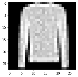
    plt.imshow(train_images[i], cmap='gray')
    plt.title(class_names[train_labels[i]])
plt.show()

• 3. Data 전처리
  데이터 다운받아 => 데이터 전처리 => 데이터셋을 만들어서 모델을 만들었을 때 데이터 넣어주는 부분을 만드는 것

# 데이터 다운받아 => 데이터 전처리 => 데이터셋을 만들어서 모델을 만들었을 때 데이터 넣어주는 부분을 만드는 것

# image를 0~1사이 값으로 만들기 위하여 255로 나누어줌
train_images = train_images.astype(np.float32) / 255. #전처리는 간단하게 이미지를 255로 나눠주는 것을 많이 사용함, 원래 이미지 픽셀값이 0~255 정수값으로 되어 있는데 이를 255로
                                                      #나눠주면 0~1사이 값으로 변경됨
                                                      #astype은 type cast(tf.cast)하는 것과 똑같음, 트레인이미지를 floating 타입으로 바꾸세요
test_images = test_images.astype(np.float32) / 255.

train_labels[0] #9

• 원핫인코딩 One Hot Encoding: keras.utils.to_categorical

# one-hot encoding : keras.utils.to_categorical : 다 0이고 정답인 자리(train_labels[0]에서 9번자리)만 1이 되게 함
train_labels = keras.utils.to_categorical(train_labels, 10)
test_labels = keras.utils.to_categorical(test_labels, 10)

train_labels[0]
array([0., 0., 0., 0., 0., 0., 0., 0., 0., 1.], dtype=float32)

• 4. Dataset 만들기
• 모델에 공급해 줄 수 있는 데이터셋을 만든다.
• 텐서플로우 공식 홈페이지 API에 대한 설명

• https://www.tensorflow.org/api_docs/python/tf/all_symbols
• https://tensorflowkorea.gitbooks.io/tensorflow-kr/content/g3doc/api_docs/

# tf.data.Dataset.from_tensor_slices
train_dataset = tf.data.Dataset.from_tensor_slices((train_images, train_labels)).shuffle( #from_tensor_slices: 굉장히 많이 사용함, 트레인 이미지와 레이블을 묶어서 텐서 1개가 들어오게
                buffer_size=100000).batch(64) #배치는 데이터를 공급할 때, 학습할때, 한번에 여러개의 이미지를 한꺼번에 넣어주게됨, 몇개씩 넣어줄것인가   #셔프은 데이터를 매번 섞어준다. 섞어줘야 데이터 학습이 잘됨
                
test_dataset = tf.data.Dataset.from_tensor_slices((test_images, test_labels)).batch(64)
# 트레인 데이터는 셔플을 안해주면 한번(1epoch당) 데이터가 들어갈 때 또 똑같은 순서로 들어가기 때문에 문제가 될 수 있다. 학습하는데 별로 좋지 않음
# 테스트 데이터는 결과만 확인하는 것이기 때문에 굳이 셔플을 할 필요가 없음

for images, labels in train_dataset:
    print(labels) #[[0. 1. 0. 0. 0. 0. 0. 0. 0. 0.] 첫번째 이미지 들어있음
    break
#셔플이 된 상태에서 레이블이 64개가 나오는 것임
# 
# tf.Tensor(
# [[0. 1. 0. 0. 0. 0. 0. 0. 0. 0.] # 셔플이 되서 이미지 첫번째꺼
#  [0. 0. 1. 0. 0. 0. 0. 0. 0. 0.]
#  ...
#  [0. 0. 0. 0. 0. 0. 0. 0. 1. 0.]], shape=(64, 10), dtype=float32) : 64개의 레이블

# Dataset을 통해 반복하기(iterate)
# 이미지와 정답(label)을 표시합니다.
imgs, lbs = next(iter(train_dataset)) #next(iter : 이터와 넥스트를 사용하면 1개를 뽑을 수 있음 https://homzzang.com/b/py-136
print(f"Feature batch shape: {imgs.shape}")
print(f"Labels batch shape: {lbs.shape}")

img = imgs[0]
lb = lbs[0]
plt.imshow(img, cmap='gray')
plt.show()
print(f"Label: {lb}")


#Label: [0. 0. 1. 0. 0. 0. 0. 0. 0. 0.] 레이블은 2번

Feature batch shape: (64, 28, 28)
Labels batch shape: (64, 10)

Label: [0. 0. 1. 0. 0. 0. 0. 0. 0. 0.]

• 5. Custom Dataset 만들기

a = np.arange(10)
print(a) #0~9까지 데이터 

ds_tensors = tf.data.Dataset.from_tensor_slices(a) #tf.data.Dataset.from_tensor_slices이 a를 데이터셋으로 만들어줌
print(ds_tensors) #데이터셋ds

for x in ds_tensors: #for문으로 데이터를 하나씩 꺼내서
    print (x)       #배치설정을 안해줘서 1개씩 내보내줌
    #print(x.numpy())
    
[0 1 2 3 4 5 6 7 8 9]
<TensorSliceDataset element_spec=TensorSpec(shape=(), dtype=tf.int64, name=None)>
tf.Tensor(0, shape=(), dtype=int64)
tf.Tensor(1, shape=(), dtype=int64)
tf.Tensor(2, shape=(), dtype=int64)
tf.Tensor(3, shape=(), dtype=int64)
tf.Tensor(4, shape=(), dtype=int64)
tf.Tensor(5, shape=(), dtype=int64)
tf.Tensor(6, shape=(), dtype=int64)
tf.Tensor(7, shape=(), dtype=int64)
tf.Tensor(8, shape=(), dtype=int64)
tf.Tensor(9, shape=(), dtype=int64)

# data 전처리(변환), shuffle, batch 추가
ds_tensors = ds_tensors.map(tf.square).shuffle(10).batch(2) #map함수는 모든 데이터에 대헤서 이 함수를 적용해주는 것, tf.square: 텐서제곱
                                                            #10: 큐의 사이즈, 얼마나 데이터를 채워놓고 셔플을 할 것인가, 데이터가 10개이므로 10개 이상만 되면 완전 셔플이됨
                                                            #배치가 2이므로 데이터를 2개씩 잘라서 내보내줌
                                                            
for _ in range(3):              #이중루프, 바깥for문이 에폭
    for x in ds_tensors:        #안쪽for문(안쪽루프): 데이터가 10개가 다들어감, 배치가 2이므로 5번 돌면 끝남
        print(x)
    print('='*50) 

#매번 셔플이 됨 ↓

tf.Tensor([25 36], shape=(2,), dtype=int64)
tf.Tensor([4 0], shape=(2,), dtype=int64)
tf.Tensor([64 49], shape=(2,), dtype=int64)
tf.Tensor([ 1 16], shape=(2,), dtype=int64)
tf.Tensor([ 9 81], shape=(2,), dtype=int64)
==================================================
tf.Tensor([ 0 16], shape=(2,), dtype=int64)
tf.Tensor([9 1], shape=(2,), dtype=int64)
tf.Tensor([64 25], shape=(2,), dtype=int64)
tf.Tensor([36 49], shape=(2,), dtype=int64)
tf.Tensor([ 4 81], shape=(2,), dtype=int64)
==================================================
tf.Tensor([64 25], shape=(2,), dtype=int64)
tf.Tensor([ 0 36], shape=(2,), dtype=int64)
tf.Tensor([49 16], shape=(2,), dtype=int64)
tf.Tensor([ 9 81], shape=(2,), dtype=int64)
tf.Tensor([1 4], shape=(2,), dtype=int64)
==================================================

2 Model

2-1 Keras Sequential API 사용

• 가장 쉽고 기본적인 모델 만드는 방법
• 시퀀셜api로 모델을 만들 수 있으면 이것을 사용, 굳이 다른 것을 써서 어렵게 만들 필요가 없음

2-2 Keras Functional API 사용

• 다양하게 네트워크를 만들 수 있는 굉장히 자유로운 모델
  (시퀀셜 api는 벽돌처럼 일렬로 쌓여있는 모델만 만들 수 있음)

• 입력은 1개인데 왼쪽, 오른쪽으로 네트워크 연결해서 왼쪽에서도 뭔가하고 오른쪽에서도 뭔가해서 다시 합치는 형태의 네트워크 가능

2-3 Model Class Subclassing 사용

• 가장 복잡해 보이는 방법
• 파이토치는 이와 유사한 방법을 사용

3 Traning / Validation

3-1 Keras API 사용

• 가장 간단한 방법

3-2 GradientTape 사용

• tf.GradientTape() : 이미지가 들어가서 로스가 가는 길까지 쭈욱 테이프에 기록을 해놨다가 테이프를 거꾸로 감아 백프로파게이션을 한다.는 의미
• 조금 더 복잡한 방법이긴 하나 굉장히 많이 사용함

4 Model 저장하고 불러오기

4-1 parameter만 저장하고 불러오기

seq_model.save_weights('seq_model.ckpt') #저장되는 포맷: 체크포인트, 확장자명은 아무렇게 해도 되나 저장포맷이 체크포인트이기 때문에 ckpt로 정해줌
# 이것만 돌려줘도 벌써 저장이 끝난 것임

seq_model_2 = create_seq_model()
seq_model_2.compile(optimizer=tf.keras.optimizers.Adam(learning_rate),
              loss='categorical_crossentropy',
              metrics=['accuracy'])
              
seq_model_2.evaluate(test_dataset) # validation set에 대해서 하는 것을 똑같이 진행, 학습은 진행하지 않고 결과만 뽑아서 val_acc, val_loss만 확인
                                   # 학습을 하나도 안한 모델이기 떄문에 loss: 2.4391 - accuracy: 0.1570(정확도15.7%)로 엉망으로 나옴
157/157 [==============================] - 1s 3ms/step - loss: 2.4391 - accuracy: 0.1570
[2.4391350746154785, 0.15700000524520874]                    

seq_model_2.load_weights('seq_model.ckpt') #load_weights 하면 저장한 모델을 불러옴
157/157 [==============================] - 0s 2ms/step - loss: 0.3254 - accuracy: 0.8823
[0.3253735303878784, 0.8823000192642212]

4-2 Model 전체를 저장하고 불러오기

seq_model.save('seq_model') # seq_model라는 디렉토리에 생성,pb파일 형태로 저장됨

import os 
os.getcwd()
/content

!ls
checkpoint   seq_model				 seq_model.ckpt.index
sample_data  seq_model.ckpt.data-00000-of-00001

seq_model_3 = keras.models.load_model('seq_model') # 모델을 통채로 불러올 수 없으니 ??

seq_model_3.evaluate(test_dataset)
157/157 [==============================] - 1s 3ms/step - loss: 0.3254 - accuracy: 0.8823
[0.3253735303878784, 0.8823000192642212]

5 Tensorboard 사용하여 시각화하기

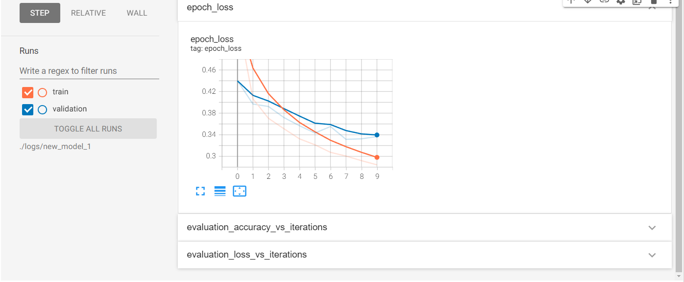
• 학습된 결과를 눈으로 보기 쉽게 해주는 시각화 툴
• 파이토치에서도 텐서보드를 사용

%load_ext tensorboard

5-1 Keras Callback 사용

new_model_1 = create_seq_model()
new_model_1.compile(optimizer=tf.keras.optimizers.Adam(learning_rate),
              loss='categorical_crossentropy',
              metrics=['accuracy'])

new_model_1.evaluate(test_dataset) #학습이 안된 상태             

157/157 [==============================] - 1s 4ms/step - loss: 2.3108 - accuracy: 0.1711
[2.3108060359954834, 0.17110000550746918]

log_dir = './logs/new_model_1' #학습되는 과정에서 w, b, loss값, acc 이런 것들을 다 저장할 경로 지정, 로그스 디렉토리에 뉴모델1번으로 저장하겠다.

tensorboard_cb = keras.callbacks.TensorBoard(log_dir, histogram_freq=1) # keras.callbacks.TensorBoard에 경로써줌, histogram_freq=1는 매 에포크마다 저장하겠다
                                                                                                                 # 매 에포크마다 w, b가 분포가 어떻게 되는지 히스토그램(그래프)로 나타냄
                                                                       new_model_1.fit(train_dataset, epochs=EPOCHS, validation_data=test_dataset,
          callbacks=[tensorboard_cb]) #callbacks이 텐서보드 말고 여러개가 있고 심지어 커스터마이즈해서 우리가 원하는 것을 만들어서 쓸수도 있음, 여러개도 들어갈 수 있음
          
Epoch 1/10
938/938 [==============================] - 4s 4ms/step - loss: 0.5584 - accuracy: 0.8051 - val_loss: 0.4398 - val_accuracy: 0.8443
Epoch 2/10
938/938 [==============================] - 3s 3ms/step - loss: 0.4065 - accuracy: 0.8536 - val_loss: 0.3968 - val_accuracy: 0.8563
Epoch 3/10
938/938 [==============================] - 4s 4ms/step - loss: 0.3704 - accuracy: 0.8664 - val_loss: 0.3923 - val_accuracy: 0.8587
Epoch 4/10
938/938 [==============================] - 3s 3ms/step - loss: 0.3511 - accuracy: 0.8732 - val_loss: 0.3718 - val_accuracy: 0.8657
Epoch 5/10
938/938 [==============================] - 3s 3ms/step - loss: 0.3324 - accuracy: 0.8785 - val_loss: 0.3567 - val_accuracy: 0.8709
Epoch 6/10
938/938 [==============================] - 3s 3ms/step - loss: 0.3214 - accuracy: 0.8813 - val_loss: 0.3431 - val_accuracy: 0.8781
Epoch 7/10
938/938 [==============================] - 3s 3ms/step - loss: 0.3074 - accuracy: 0.8874 - val_loss: 0.3553 - val_accuracy: 0.8728
Epoch 8/10
938/938 [==============================] - 3s 3ms/step - loss: 0.3006 - accuracy: 0.8896 - val_loss: 0.3315 - val_accuracy: 0.8821
Epoch 9/10
938/938 [==============================] - 4s 4ms/step - loss: 0.2920 - accuracy: 0.8920 - val_loss: 0.3324 - val_accuracy: 0.8835
Epoch 10/10
938/938 [==============================] - 5s 5ms/step - loss: 0.2843 - accuracy: 0.8947 - val_loss: 0.3367 - val_accuracy: 0.8794
<keras.callbacks.History at 0x7fedba7aa1d0>                                                                                                     %tensorboard --logdir $log_dir #%: 매직커맨드, 원래 텐서보드는 인터넷 익스플로어나 크롬창에 띄어서 보는 건데 여기 아래 그냥 볼수도 있음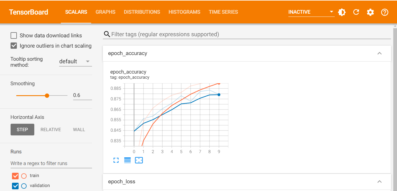            

5-2 Summary Writer 사용

new_model_2 = create_seq_model()

# loss function
loss_object = keras.losses.CategoricalCrossentropy()

# optimizer
learning_rate = 0.001
optimizer = keras.optimizers.Adam(learning_rate=learning_rate)

# loss, accuracy 계산
train_loss = keras.metrics.Mean(name='train_loss')
train_accuracy = keras.metrics.CategoricalAccuracy(name='train_accuracy')

test_loss = keras.metrics.Mean(name='test_loss')
test_accuracy = keras.metrics.CategoricalAccuracy(name='test_accuracy')

@tf.function
def train_step(model, images, labels):
  with tf.GradientTape() as tape:
    # training=True is only needed if there are layers with different
    # behavior during training versus inference (e.g. Dropout).
    predictions = model(images, training=True)
    loss = loss_object(labels, predictions)
  gradients = tape.gradient(loss, model.trainable_variables)
  optimizer.apply_gradients(zip(gradients, model.trainable_variables))

  train_loss(loss)
  train_accuracy(labels, predictions)
  
@tf.function
def test_step(model, images, labels):
  # training=False is only needed if there are layers with different
  # behavior during training versus inference (e.g. Dropout).
  predictions = model(images, training=False)
  t_loss = loss_object(labels, predictions)

  test_loss(t_loss)
  test_accuracy(labels, predictions)
  
import datetime

current_time = datetime.datetime.now().strftime("%Y%m%d-%H%M%S") #디렉터리를 시간에 따라 다르게 함
train_log_dir = 'logs/gradient_tape/' + current_time + '/train'
test_log_dir = 'logs/gradient_tape/' + current_time + '/test'
train_summary_writer = tf.summary.create_file_writer(train_log_dir)
test_summary_writer = tf.summary.create_file_writer(test_log_dir)  

EPOCHS = 10

for epoch in range(EPOCHS):
  # Reset the metrics at the start of the next epoch
  train_loss.reset_states()
  train_accuracy.reset_states()
  test_loss.reset_states()
  test_accuracy.reset_states()

  for images, labels in train_dataset:
    train_step(new_model_2, images, labels)
  with train_summary_writer.as_default():
    tf.summary.scalar('loss', train_loss.result(), step=epoch)  #tf.summary.scalar라고 써주면 loss와 acc저장됨, tf.summary.histogram 도 쓸 수 있음
    tf.summary.scalar('accuracy', train_accuracy.result(), step=epoch)

  for test_images, test_labels in test_dataset:
    test_step(new_model_2, test_images, test_labels)
  with test_summary_writer.as_default():
    tf.summary.scalar('loss', test_loss.result(), step=epoch)
    tf.summary.scalar('accuracy', test_accuracy.result(), step=epoch)

  print(
    f'Epoch {epoch + 1}, '
    f'Loss: {train_loss.result()}, '
    f'Accuracy: {train_accuracy.result() * 100}, '
    f'Test Loss: {test_loss.result()}, '
    f'Test Accuracy: {test_accuracy.result() * 100}'
  )
  
Epoch 1, Loss: 0.5604304075241089, Accuracy: 80.38166809082031, Test Loss: 0.4423648416996002, Test Accuracy: 84.26000213623047
Epoch 2, Loss: 0.41018834710121155, Accuracy: 85.15999603271484, Test Loss: 0.3988458812236786, Test Accuracy: 85.62999725341797
Epoch 3, Loss: 0.37535423040390015, Accuracy: 86.41832733154297, Test Loss: 0.3675061762332916, Test Accuracy: 86.73999786376953
Epoch 4, Loss: 0.3489702045917511, Accuracy: 87.38500213623047, Test Loss: 0.3603389859199524, Test Accuracy: 87.05999755859375
Epoch 5, Loss: 0.3366009294986725, Accuracy: 87.65499877929688, Test Loss: 0.37690696120262146, Test Accuracy: 86.11000061035156
Epoch 6, Loss: 0.31973475217819214, Accuracy: 88.3183364868164, Test Loss: 0.3514719605445862, Test Accuracy: 87.25
Epoch 7, Loss: 0.308842271566391, Accuracy: 88.50499725341797, Test Loss: 0.3435555100440979, Test Accuracy: 87.52999877929688
Epoch 8, Loss: 0.300233393907547, Accuracy: 88.86333465576172, Test Loss: 0.3475845456123352, Test Accuracy: 87.12000274658203
Epoch 9, Loss: 0.29194337129592896, Accuracy: 89.09666442871094, Test Loss: 0.3521362245082855, Test Accuracy: 87.47000122070312
Epoch 10, Loss: 0.284616619348526, Accuracy: 89.43333435058594, Test Loss: 0.33865824341773987, Test Accuracy: 87.98999786376953  

%tensorboard --logdir 'logs/gradient_tape'