Semi-Supervised Classification with Graph Convolutional Networks

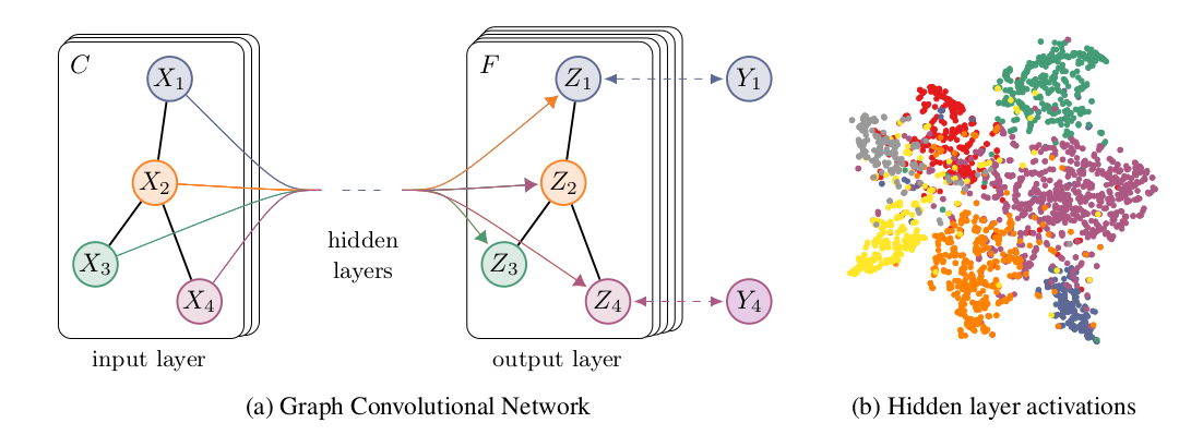
드디어 ASCO 학회 제출이 끝났다! 조금 여유가 생기기도 했고 graph 쪽을 전부터 공부해보고 싶었는데 마침 동료분이 graph 사용해서 whole slide image 분석하는 모델 시도해 보신다고 해서 겸사겸사 나도 시작했다. Graph 쪽 처음 본 논문은 사실 이 논문이 아니라 nature biomedical 논문인데 그건 다음 논문리뷰로 작성해보도록 하겠다. 이번 논문 GCN 은 spectral 관점에서 graph node 간의 관계를 고려해서, node 가 가지고 있는 feature 를 layer 에 통과시켜 각 노드가 어떤 class 에 해당하는지 분류하는 문제를 푸는 연구를 담고 있다.

Introduction

graph data 특성 상 각 node 마다 label 이 매우 적게 존재하기 때문에 graph node classification problem 은 보통 semi-supervised learning 으로 frame 된다. 기존 방식들은 label 이 존재하는 데이터에 대해 loss 를 따로 계산하고, label 이 존재하지 않는 데이터에 대해 graph Laplacian regularization term 을 이용해서 다음과 같이 계산해 왔었다.

하지만 이 regularization term 은 "노드 사이의 거리가 가까우면, feature 가 비슷할 것이다" 라는, 다소 다른 추가적인 정보를 버릴 위험이 있는 term 이기 때문에, 저자는 이러한 term (explicit graph-based regularization) 사용을 지양하고자 하였다.

이들의 contribution 은 다음으로 요약할 수 있다.

• introduce simple and well-behaved layer-wise propagation rule for NN moel which operate directly on graphs
  -> how it can be motivated from a first-order approximation of spectral graph convolutions
• demonstrate speed and scalability in semi-supervised classification of nodes in a graph

Background, notes

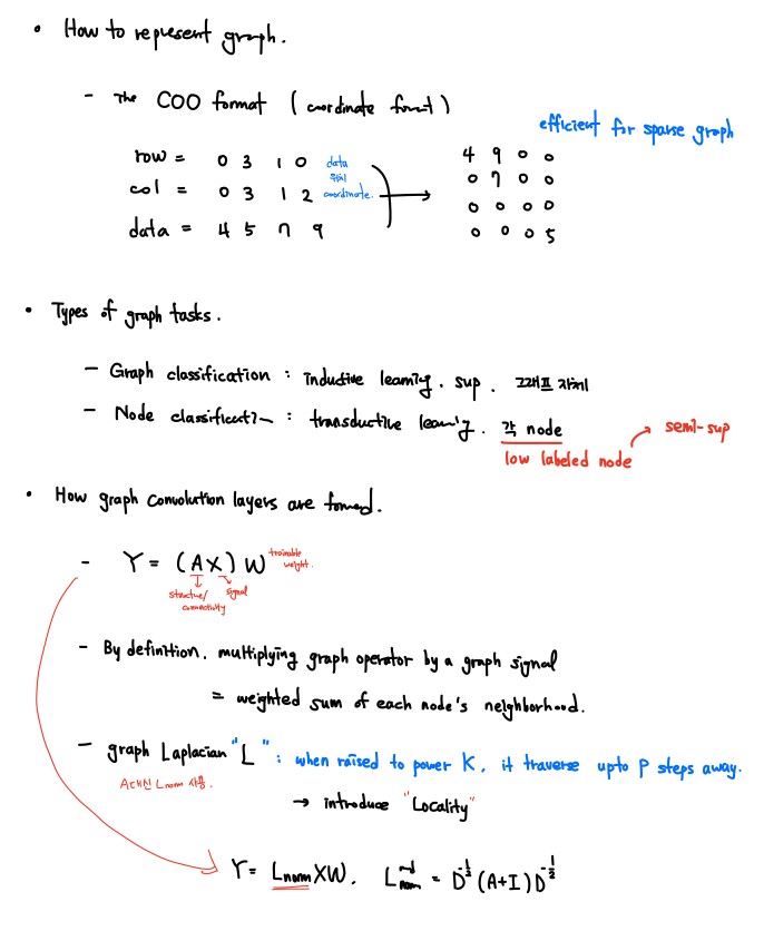
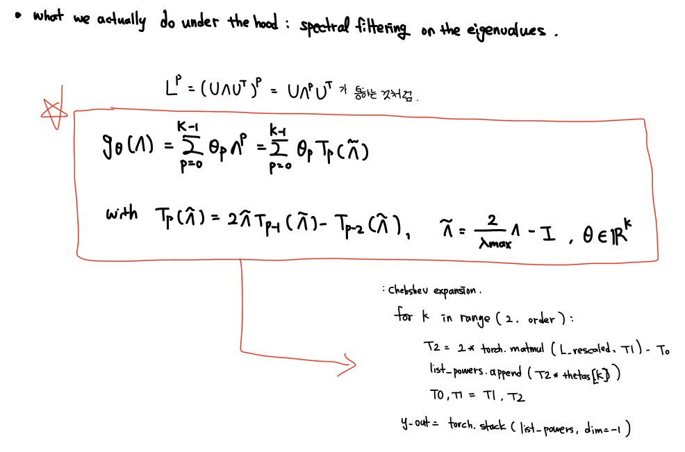
여기부터는 그 전 논문들에서 다루고 있는 spectral graph convolution 에 대한 이해가 필요하다. 따라서 논문의 내용을 설명하기 전 다음 블로그를 참고하여 정리한 노트를 첨부한다. 노트의 Chebyshev expansion 까지가 background 이고, reparameterization 및 rescaling 등의 trick 은 이번 GCN 논문에서 소개된다.

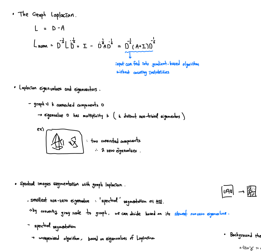
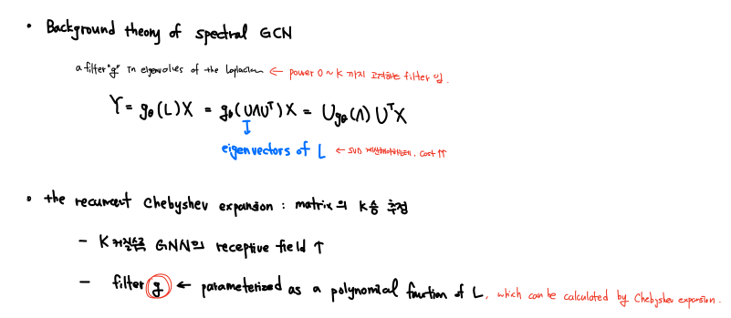
이 때, computationally expensive 하기 때문에 Chebyshev polynomial 을 사용한다.

출처: https://theaisummer.com/graph-convolutional-networks/

Fast Approximate Convolutions on Graphs

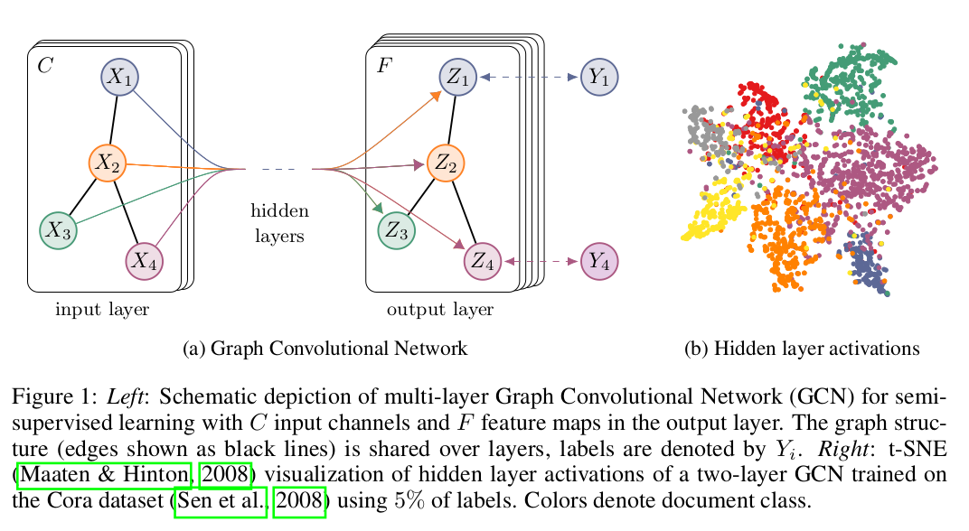
multi-layer Graph Convolutional Network (GCN) 은 다음과 같은 layer-wise propagation rule 로 정의된다.

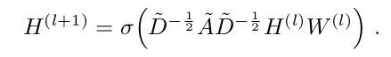
이 때 A는 self-connection 이 추가된 adjacency matrix 이고, D는 self-connection 이 추가된 A의 D이다. non linear function 은 ReLU function 을 사용했고, $H^{(l)}$ 은 N x D l번째 layer 을 뜻하며, 이에 상응하여 $H^{(0)}$ 은 데이터 그 자체 $x \in$ N 이다

Spectral Graph Convolutions

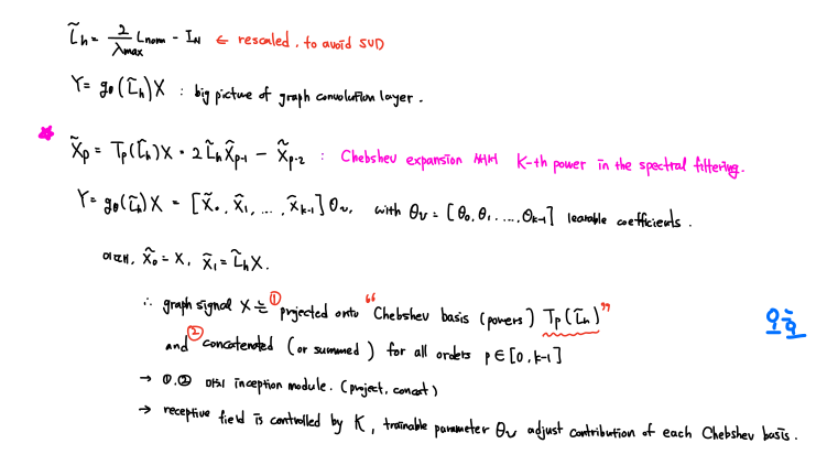
x 라는 graph signal 에 $g_{\theta}=diag(\theta)$ filter parameterized by $\theta \in \real^N$ in Fourier domain 를 붙인 형태로, spectral convolution 이 정의된다. ex)

이 때, U 는 normalized graph Laplacian 의 eigenvector 이고, eigenvalue 는 graph Fourier transform of x 가 된다. 하지만 이런 방식을 사용하면, 1) L 에 대해 SVD 를 적용해야 하고 2) eigenvalue matrix U 를 multiplication 해야 함으로 computation cost 가 크다. 이러한 문제점을 극복하기 위해, 이전에 Chebyshev expansion 을 사용하여 series 형태로 각 locality 에 해당하는 filter 통과 feature $T_k(x)$ 의 합을 다음과 같이 표현했다.

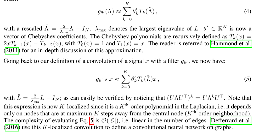
여기까지 사전지식에 해당한다. 각 locality k 에 대해 계산된 filter 를 통과한 feature 들이 concat 된 형태로, inception module 과 닮아있다.

Layer-wise Linear Model

위에서 한 layer 를 표현했기 때문에, neural network model 도 convolution layer 형태를 띈 Equation (5) 를 여러개 stacking 함으로써 만들어 낼 수 있다. 이 때 한 layer 를 정의하기 위해, $\lambda_{max}$ 가 대략 2라고 가정하고 K=1 인 경우를 생각해보면, free parameter $\theta'_0,\theta'_1$ 와 함께 다음처럼 표현된다.

이 때, filter parameter 는 whole graph 에서 share 가능한 형태이므로, successive application of filter 를 stack 해서 사용하다면, kth - order neighborhood of node 를 표현할 수 있게 되는 것이다. (위에서 k 는 locality 라고 표현했었음.)

또한 실용적인 측면에서 저자는 새로운 renormalization trick 을 제안한다. 두개의 free parameter 값을, 두 parameter 간의 관계를 정의함으로써 하나로 변경하고 표현하면 다음과 같이 표현된다.

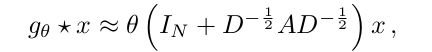
이 때, 가운데 In+DAD 항은 가정된 대로 0-2 사이의 eigenvalue 값을 가지게 되는데, repeated application 을 거치면 numerical instability 와 exploding/vanishing gradient 를 초래할 수 있다. 이를 해결하기 위해,

다음과 같은 renormalization 과정을 거쳐, 다음과 같은 일반적인 형태를 얻도록 하였다.

Semi-Supervised Node Classification

위에서 언급한 구조를 정리하면 다음과 같다.

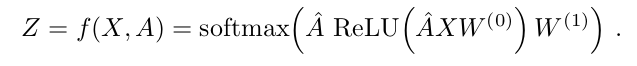
이 때 loss 는 labeled examples 에 대해서 cross-entropy 형태로 사용한다.

Experiment & Result

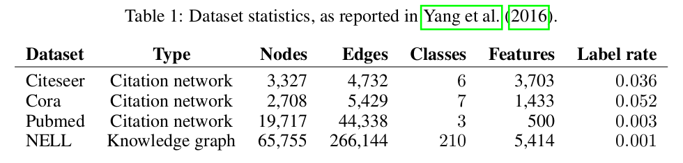
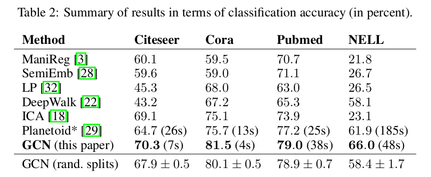
3개의 citation network 에서의 document classification task 로 수행하였다.
Dataset 은 다음과 같다.

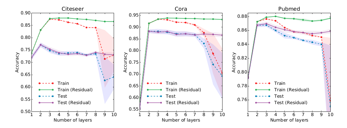
model 은 기본적으로 2-layer shallow network 를 사용하였고, supplementary result 에 layer 개수를 늘린 실험 결과를 나타내었다.
1000개의 labeled example 로 test 하였고, 여러 baseline 과 함께 성능을 기록하였다.

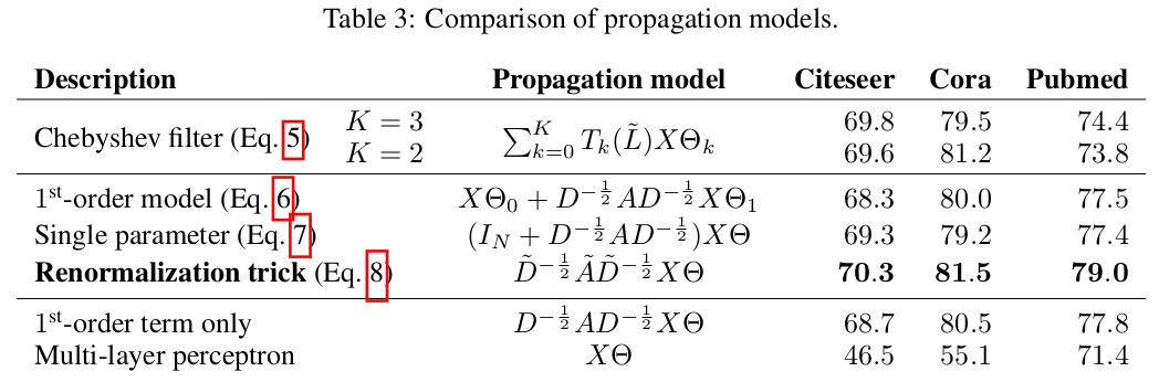
다른 propagation logic 을 사용해서 성능을 비교하였다.

Discussion

다음과 같은 한계점을 언급하였다.

• Memory requirement grows linearly in the size of the dataset
• Directed edges and edge features are limited
• Limiting assumptions
  --> self connection 과 edge 간의 importance 를 동일하게 취급함.
  --> implicit하게 locality 를 가정함. (Kth layer 는 Kth order neighborhood이다.)

재밌구만